
Section 10.4 Parts of a Quarto document

Quarto documents are similar to R scripts, but they have more rules and structure. Here, we will be breaking down the different sections.

Subsection 10.4.1 The YAML

At the top of the document you will find what is called the YAML, which contains the metadata for the document. When you first open a new Quarto Document, it looks like this:
---
title: "Untitled"
format: html
editor: visual
---
It has four default components:
  • title: What the title of your Quarto is.
  • format: The output you designated the document to be created into
    • There are some cool things you can add here, like change the overall theme or add TOC (table of contents). Like anything in R, take some time to explore and experiment with this.
  • editor: tells Quarto (and RStudio) to open the document in the Visual Editor by default, instead of the Source Editor (more about this in SubsectionΒ 10.4.2).
You’ll also notice that the YAML is contained within ---. Besides being at the top of the document, this is Quarto’s way of knowing that this specific part of the document is the YAML.

Subsection 10.4.2 Source and Visual Panes

In a traditional R script, all of your code is written (for the most part) in the source quadrant (see SectionΒ 1.2). If you look towards the top left of the Quarto document, you can see that there are two options adjacent to each other: Source and Visual. Amazingly, Quarto allows you to view what your document looks like in a published format using the Visual pane.
For the most part, anything you can do in one view can be done in the other. Source looks more like an R script, while Visual looks more like a traditional document. I highly suggest playing around and experimenting in both to see the interactivity and capabilities.
There are no wrong answers!

Subsection 10.4.3 Text

In an R script, every line is dedicated to writing code, with you having to specifically use a # to denote otherwise (as a reminder, in R code, a # comments out whatever is on that line, whether code or text). That is different in Quarto.
Instead of the default being R code, anything you write in a document is treated as text. This is incredibly useful when you want to:
For instance, what you’re reading right now is text inside a Quarto document. There is no special way of telling Quarto that this content is text, because text is the default.
There are, though, ways to tell Quarto how to format text.

Subsubsection 10.4.3.1 Styling Text

Just like in any document, sometimes we want to make particular pieces of text look different. The two most common ways to style text in Quarto are:
Italic: to do this, add * to the beginning and end of your text (whether a single letter, word, sentence, paragraph, etc.).
*It will look like this.*
Bold: to do this, add ** to the beginning and end of your text (whether a single letter, word, sentence, paragraph, etc.).
**It will look like this.**
These are the two basic ways to edit text. What if we need to indent in order to create a list?

Subsubsection 10.4.3.2 Adding Lists

As with traditional documents, Quarto is able to create lists, whether that is numbered or bulleted. In order to create a bulleted list, a - and then a space between the text is needed. For a numbered list, you need the number, then a period, then a space before your text. Below are examples of both.
- Text
- More text

1. Text
2. More text
We have seen both of these ample times throughout this textbook, and also in this chapter!
Now that we have talked more about the text portions of a Quarto, let’s now talk about the code portions.

Subsection 10.4.4 R chunks

Similar to how the YAML used the --- to enclose whatever was inside, for R chunks, Quarto uses "```". Whatever is inside an R chunk is treated as R code.
Additionally, each R chunk has {}, and inside of that bracket is the letter "r". This tells Quarto to run the chunk as R code.
It is typically best practice to also name your R chunks. Each one should be a unique name, not only for a way for you to distinguish them from each other, but for R to distinguish them as well. To name your R chunk, you will use the #| (called the hash-pipe) and then the label:.

What is the #| anyway?

In Quarto, that is used to give information regarding the R chunk, and tells Quarto that anything on this line is not R code to run.
For example, the below code would name an R chunk "r-is-awesome."
#| label: r-is-awesome
It is best practice to either use one long word or use a - in between your words. In each Quarto document, there are two major types of R chunks.

Subsubsection 10.4.4.1 Chunks for R Code

It has already been established that in order to write R code, you need to create an R chunk. Inside an R chunk, you are able to code as normally as you would in an R script. The same rules (even adding comments) apply inside an R chunk. Think of each R chunk as a mini R script.
Take the code below. This, as well as all of the code in the book is written inside R chunks. Below is some code that is from all the way back from section SubsectionΒ 2.5.8 of the book.
library(tidyverse)
library(palmerpenguins)

penguins_new <- penguins |>
  select(species, island, bill_length_mm, body_mass_g) |>
  filter(species == "Adelie") |>
  mutate(size_category = if_else(body_mass_g >= 3500, "Big","Small")) |>
  arrange(desc(body_mass_g)) |>
  rename(penguin_types = species)
This code works just as it did in the third chapter. In the Quarto document, all of the code shows. This is an example of how now, for anyone looking, they are able to see your code.
What if we want them to see not only the code, but the output? All we have to do is call what we want to be displayed! For instance, if we want to display the square root of 25 (like in SubsectionΒ 1.3.2):
sqrt(25)
[1] 5
With the above R code, our Quarto document shows both the sqrt(25) code as well as the answer (5).
This is the same no matter if it is square root, ANOVAs, linear regressions, and anything else in this chapter.
Naming your R chunks:.
Part of making your document reproducible is making sure people can follow along, and part of that is naming your R chunks. To do this, you can use the following: #| label:. The #| lets R know that the information is related to the chunk itself and is not R code, while label: allows you to name the R chunk. You can name it whatever you want, for example:
#| label: first-R-chunk
If your R chunk has a table or graph that will be displayed, you need to tell R that by providing prefixes to your label names. They are as follows:
Now let’s move on to displaying tables and graphs.
Tables.
Let’s go back to that penguins_new dataset. Before in section SubsubsectionΒ 10.4.4.1, we "created" it. Now, let’s see what happens when we call the output.
penguins_new
# A tibble: 152 Γ— 5
   penguin_types island    bill_length_mm body_mass_g size_category
   <fct>         <fct>              <dbl>       <int> <chr>        
 1 Adelie        Biscoe              43.2        4775 Big          
 2 Adelie        Biscoe              41          4725 Big          
 3 Adelie        Torgersen           42.9        4700 Big          
 4 Adelie        Torgersen           39.2        4675 Big          
 5 Adelie        Dream               39.8        4650 Big          
 6 Adelie        Dream               39.6        4600 Big          
 7 Adelie        Biscoe              45.6        4600 Big          
 8 Adelie        Torgersen           42.5        4500 Big          
 9 Adelie        Dream               37.5        4475 Big          
10 Adelie        Torgersen           41.8        4450 Big          
# β„Ή 142 more rows
By calling penguins_new, the Quarto document now displays the output, which in this case is penguins_new.
Naming Table Chunks:.
To let Quarto know that there is a table in your R chunk that you are going to display, make sure its name starts with tbl-.
#| label: tbl-penguins_new_display
#| tbl-cap: "Showing what a plain table looks like in a Quarto document."
penguins_new
# A tibble: 152 Γ— 5
   penguin_types island    bill_length_mm body_mass_g size_category
   <fct>         <fct>              <dbl>       <int> <chr>        
 1 Adelie        Biscoe              43.2        4775 Big          
 2 Adelie        Biscoe              41          4725 Big          
 3 Adelie        Torgersen           42.9        4700 Big          
 4 Adelie        Torgersen           39.2        4675 Big          
 5 Adelie        Dream               39.8        4650 Big          
 6 Adelie        Dream               39.6        4600 Big          
 7 Adelie        Biscoe              45.6        4600 Big          
 8 Adelie        Torgersen           42.5        4500 Big          
 9 Adelie        Dream               37.5        4475 Big          
10 Adelie        Torgersen           41.8        4450 Big          
# β„Ή 142 more rows
Now, that works, but in Quarto, there is an even better way to display tables. Using the knitr package ([D.1.13]), we can display tables with the kable() function, which is purposely dedicated to displaying tabular data in Quarto.
Displaying Tables with kable().
Throughout this book, we often use the kable() function to format tables for display in Quarto. This improves readability and ensures tables render cleanly in the final document.
However, kable() is not required when working interactively in R. The underlying objects (data frames, matrices, model summaries) can always be printed directly. We use kable() here purely for presentation purposes.
If you want to get even fancier, you can always use some functions within the kableExtra package.
#| label: tbl-penguins_new_display_kable
library(knitr)
kable(head(penguins_new), caption = "This is an example of displaying a table using the kable command. On top of the data looking nicer than just a regular output, we can add a caption (and manipulate other aesthetic pieces.")
Table: This is an example of displaying a table using the kable command. On top of the data looking nicer than just a regular output, we can add a caption (and manipulate other aesthetic pieces.

|penguin_types |island    | bill_length_mm| body_mass_g|size_category |
|:-------------|:---------|--------------:|-----------:|:-------------|
|Adelie        |Biscoe    |           43.2|        4775|Big           |
|Adelie        |Biscoe    |           41.0|        4725|Big           |
|Adelie        |Torgersen |           42.9|        4700|Big           |
|Adelie        |Torgersen |           39.2|        4675|Big           |
|Adelie        |Dream     |           39.8|        4650|Big           |
|Adelie        |Dream     |           39.6|        4600|Big           |
If we compare and contrast the output from just penguins_new vs the output from the kable() function, there is a stark difference. One of the most important differences is that you can add a caption that can illuminate the table more than just a simple output.
Captions with tables:.
You could create a caption for your table using #| tbl-cap: if you were not using kable(). However, it is best practice to use kable().
In the code above, we could have just called penguins_new and not just the head() of penguins_new, so why did we do this?
If we did not call head() then kable() would have produced a table displaying all rows from penguins_new, which would have the user scrolling for a long time. It is always your call as the creator of the document, but keep this in mind:
By calling head(), your audience still gets a good picture of what your data looks like.
Graphs.
In Quarto, just how we can display tables, we can also display graphs.
Naming Graph Chunks:.
To let Quarto know that there is a graph in your R chunk that you are going to display, make sure its name starts with fig-.
Similar to working with tables, when working with graphs and you want to add a caption, you can use fig-cap: on a line with the #|.
#| label: fig-example-ggplot2
#| fig-cap: "An example of a visualization made using ggplot2."
library(ggplot2)
ggplot(data = mpg, aes(x = cty, y = hwy)) +
  geom_point()
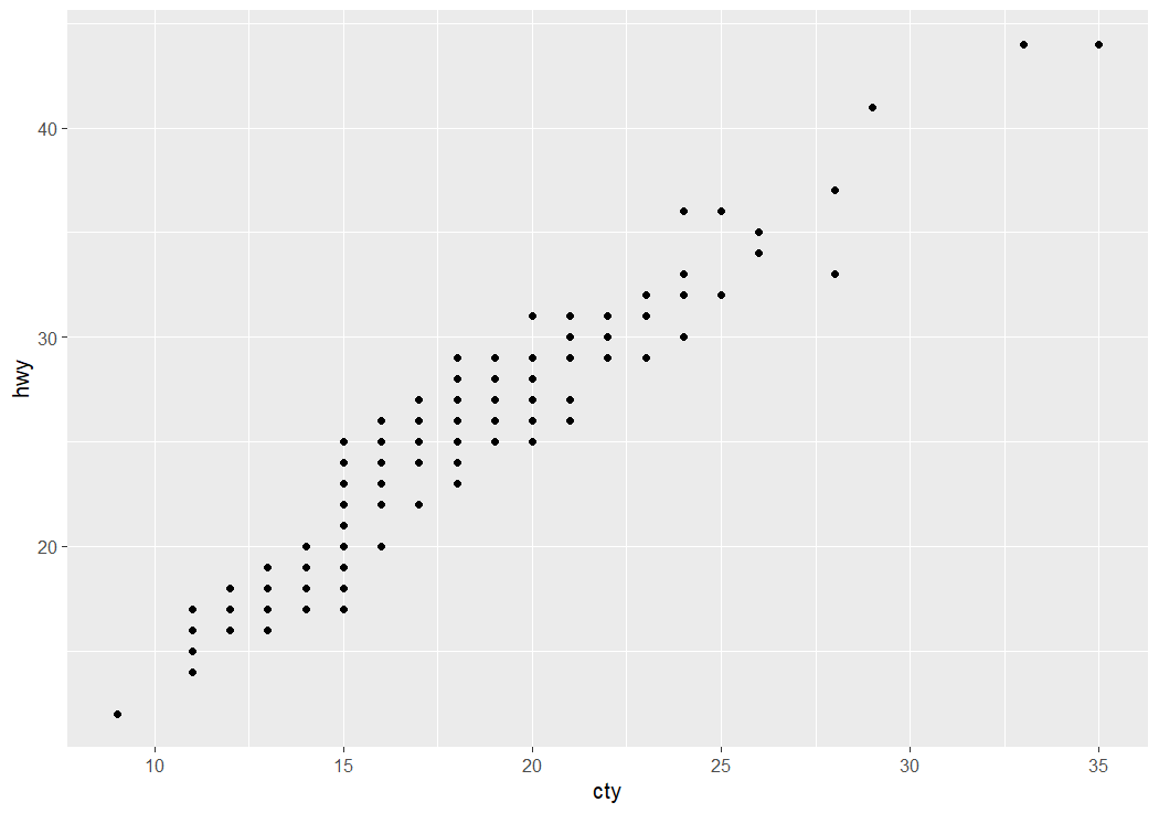
A scatterplot with city mileage on the x-axis and highway mileage on the y-axis, showing a positive relationship between the two variables across 234 vehicles in the mpg dataset.
Figure 10.4.1. An example of a visualization made using ggplot2. This scatterplot displays the relationship between city mileage (cty) and highway mileage (hwy) from the mpg dataset.
This visualization, which we originally built in Section SubsectionΒ 3.4.2, not only displays the data, but provides a caption to explain the visualization, all thanks to fig-cap:.
Yes, a picture is worth 1,000 words, but sometimes it can be helpful to add some words to help guide viewers.

Subsection 10.4.5 Sections

One of the most important and powerful parts of a Quarto document is its ability to organize elements into Sections.
Do you see how this chapter, and each chapter of the textbook, are broken down into sections like 10.1, 3.7, etc? Each number represents a different section of the document.
Quarto utilizes the # symbol to set up sections. Here is an example:
# Section 1
# Section 2
## Section 2.1
Notice that a hierarchy is determined through the number of # in the header. Each additional # means one level lower.
Headers, just like R chunks, also need labeling. To do that, inside {} on the same line as the header, add a # within the {} followed up whatever name you want. Just how tables and graphs have specific prefixes, so do section headers, which is sec-. An example of a section name is as follows:
{#sec-creating-sections}

Label Correctly!

Use proper naming convention when naming anything inside your Quarto document.
Lets see why naming is so important in a practical sense.

Subsection 10.4.6 Cross-Referencing Syntax

I have been emphasizing how important it is to properly name thingsβ€”whether it is headings, tables, or figures. Naming is vital for organization and reproducibility, but it is also the "secret sauce" for cross-referencing within Quarto documents.
For instance, back in Graphs, we created the example ggplot2 figure.
That right there is a cross-reference. By typing @fig-example-ggplot2 in my text, Quarto automatically turned it into a clickable link, with the @ symbol being the driving factor. It even indexes the figures based on the order they’re created. If I were to add another graph earlier in the chapter, Quarto would automatically update the numbering so this one becomes "Figure 2" without me having to change a thing.


Labeling is Key!

This can only be done with proper naming convention, so make sure to properly label your tables and graphs!