Skip to main content
Contents Index Dark Mode Prev Up Next \(\require{cancel}
\newcommand{\lt}{<}
\newcommand{\gt}{>}
\newcommand{\amp}{&}
\definecolor{fillinmathshade}{gray}{0.9}
\newcommand{\fillinmath}[1]{\mathchoice{\colorbox{fillinmathshade}{$\displaystyle \phantom{\,#1\,}$}}{\colorbox{fillinmathshade}{$\textstyle \phantom{\,#1\,}$}}{\colorbox{fillinmathshade}{$\scriptstyle \phantom{\,#1\,}$}}{\colorbox{fillinmathshade}{$\scriptscriptstyle\phantom{\,#1\,}$}}}
\)
Section 1.2 RStudio
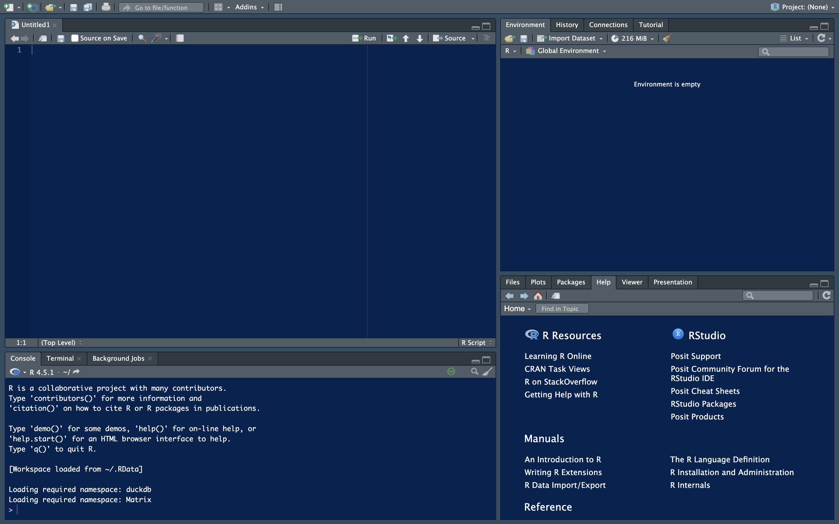
Currently we are using RStudio to run R.
Figure 1.2.1. A picture of the RStudio quadrants
Here, there are 4 quadrants/panes
This is where 99% of all of your code will be written.
This is where we will see if our code ran or if we have errors. That remaining 1% of code written from before will be done here.
This is where you see what is being stored in your environment, such as data, values, and functions.
Files/Plots/Packages/etc - bottom right
There are many tabs here, which are mostly self-explanatory
Don’t panic if your screen looks different! You can click and drag the panes to rearrange them, but the
names of the quadrants (Source, Console, Environment, Files) will always be the same.
Now that we know what we are looking at, let’s get into some R code!
It was explained that a vast majority of our code will be written in the source quadrant, specifically, in an
R Script . Once R Studio has been opened, you can go to file, file new, then click on R Script. A brand new R Script has now been opened for you to begin your coding adventure!