A Population

Section 4.3 A Population

In this section we introduce the variability of a population and present some numerical summaries that characterizes this variability. Before doing so, let us review with the aid of an example some of the numerical summaries that were used for the characterization of the variability of data.

🔗

Recall the file “ex1.csv” that contains data on the height and sex of 100 subjects. (The data file can be obtained from http://pluto.huji.ac.il/~msby/StatThink/Datasets/ex1.csv.) We read the content of the file into a data frame by the name “ex.1” and apply the function “summary” to the data frame:

🔗

ex.1 <- read.csv("_data/ex1.csv")
summary(ex.1)

##        id              sex         height     
##  Min.   :1538611   FEMALE:54   Min.   :117.0  
##  1st Qu.:3339583   MALE  :46   1st Qu.:158.0  
##  Median :5105620               Median :171.0  
##  Mean   :5412367               Mean   :170.1  
##  3rd Qu.:7622236               3rd Qu.:180.2  
##  Max.   :9878130               Max.   :208.0

We saw in the previous chapter that, when applied to a numeric sequence, the function “summary” produces the smallest and largest values in the sequence, the three quartiles (including the median) and the mean. If the input of the same function is a factor then the outcome is the frequency in the data of each of the levels of the factor. Here “sex” is a factor with two levels. From the summary we can see that 54 of the subjects in the sample are female and 46 are male.

🔗

Notice that when the input to the function “summary” is a data frame, as is the case in this example, then the output is a summary of each of the variables of the data frame. In this example two of the variables are numeric (“id” and “height”) and one variable is a factor (“sex”).

🔗

Recall that the mean is the arithmetic average of the data which is computed by summing all the values of the variable and dividing the result by the number of observations. Hence, if $n$ is the number of observations ($n=100$ in this example) and $x_i$ is the value of the variable for subject $i\text{,}$ then one may write the mean in a formula form as

🔗

\begin{equation*} \bar x = \frac{\mbox{Sum of all values in the data}}{\mbox{Number of values in the data}} = \frac{\sum_{i=1}^n x_i}{n}\;, \end{equation*}

where $\bar x$ corresponds to the mean of the data and the symbol “$\sum_{i=1}^n x_i$” corresponds to the sum of all values in the data.

🔗

The median is computed by ordering the data values and selecting a value that splits the ordered data into two equal parts. The first and third quartile are obtained by further splitting each of the halves into two quarters.

🔗

Let us discuss the variability associated with an entire target population. The file “pop1.csv” that contains the population data can be found on the internet (http://pluto.huji.ac.il/~msby/StatThink/Datasets/pop1.csv). It is a CSV file that contains the information on sex and height of an entire adult population of some imaginary city. (The data in “ex.1” corresponds to a sample from this city.) Read the population data into R and examine it:

🔗

pop.1 <- read.csv(file="_data/pop1.csv")
summary(pop.1)

##        id              sex            height   
##  Min.   :1000082   FEMALE:48888   Min.   :117  
##  1st Qu.:3254220   MALE  :51112   1st Qu.:162  
##  Median :5502618                  Median :170  
##  Mean   :5502428                  Mean   :170  
##  3rd Qu.:7757518                  3rd Qu.:178  
##  Max.   :9999937                  Max.   :217

The object “pop.1” is a data frame of the same structure as the data frame “ex.1”. It contains three variables: a unique identifier of each subject (id), the sex of the subject (sex), and its height (height). Applying the function “summary” to the data frame produces the summary of the variables that it contains. In particular, for the variable “sex”, which is a factor, it produces the frequency of its two categories — 48,888 female and 51,112 — a total of 100,000 subjects. For the variable “height”, which is a numeric variable, it produces the extreme values, the quartiles, and the mean.

🔗

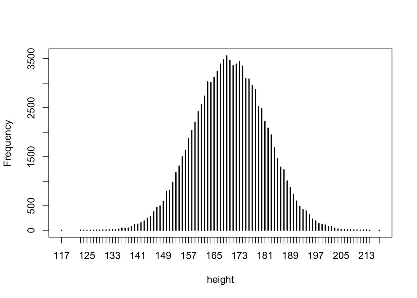
Bar plot showing the distribution of heights in the population, with heights ranging from 117 to 217 centimeters and centered at 170 centimeters — Figure 4.3.1. Bar Plot of Height
🔗

Let us concentrate on the variable “height”. A bar plot of the distribution of the heights in the entire population is given in Figure 4.3.1

Such a bar plot can be produced with the expression “plot(table(pop.1$height))”.

. Recall that a vertical bar is placed above each value of height that appears in the population, with the height of the bar representing the frequency of the value in the population. One may read out of the graph or obtain from the numerical summaries that the variable takes integer values in the range between 117 and 217 (heights are rounded to the nearest centimeter). The distribution is centered at 170 centimeter, with the central 50% of the values spreading between 162 and 178 centimeters.

🔗

The mean of the height in the entire population is equal to 170 centimeter. This mean, just like the mean for the distribution of data, is obtained by the summation of all the heights in the population divided by the population size. Let us denote the size of the entire population by $N\text{.}$ In this example $N = 100,000\text{.}$ (The size of the sample for the data was called $n$ and was equal to $n=100$ in the parallel example that deals with the data of a sample.) The mean of an entire population is denoted by the Greek letter $\mu$ and is read “mew”. (The average for the data was denoted $\bar x$). The formula of the population mean is:

🔗

\begin{equation*} \mu = \frac{\mbox{Sum of all values in the population}}{\mbox{Number of values in the population}}= \frac{\sum_{i=1}^N x_i}{N}\;. \end{equation*}

Observe the similarity between the definition of the mean for the data and the definition of the mean for the population. In both cases the arithmetic average is computed. The only difference is that in the case of the mean of the data the computation is with respect to the values that appear in the sample whereas for the population all the values in the population participate in the computation.

🔗

In actual life, we will not have all the values of a variable in the entire population. Hence, we will not be able to compute the actual value of the population mean. However, it is still meaningful to talk about the population mean because this number exists, even though we do not know what its value is. As a matter of fact, one of the issues in statistics is to try to estimate this unknown quantity on the basis of the data we do have in the sample.

🔗

A characteristic of the distribution of an entire population is called a parameter. Hence, $\mu\text{,}$ the population average, is a parameter. Other examples of parameters are the population median and the population quartiles. These parameters are defined exactly like their data counterparts, but with respect to the values of the entire population instead of the observations in the sample alone.

🔗

Another example of a parameter is the population variance. Recall that the sample variance was defined with the aid of the deviations $x_i - \bar x\text{,}$ where $x_i$ is the value of the measurement for the $i$th subject and $\bar x$ is the mean for the data. In order to compute the sample variance these deviations were squared to produce the squared deviations. The squares were summed up and then divided by the sample size minus one ($n-1$). The sample variance, computed from the data, was denoted $s^2\text{.}$

🔗

The population variance is defined in a similar way. First, the deviations from the population mean $x_i - \mu$ are considered for each of the members of the population. These deviations are squared and the average of the squares is computed. We denote this parameter by $\sigma^2$ (read “sigma square”). A minor difference between the sample variance and the population variance is that for the latter we should divide the sum of squared deviations by the population size ($N$) and not by the population size minus one ($N-1$):

🔗

\begin{align*} \sigma^2 =\amp \mbox{The average square deviation in the population}\\ =\amp \frac{\mbox{Sum of the squares of the deviations in the population}}{\mbox{Number of values in the population}}\\ =\amp \frac{\sum_{i=1}^N (x_i-\mu)^2}{N}\;. \end{align*}

The standard deviation of the population, yet another parameter, is denoted by $\sigma$ and is equal to the square root of the variance. The standard deviation summarizes the overall variability of the measurement across the population. Again, the typical situation is that we do not know what the actual value of the standard deviation of the population is. Yet, we may refer to it as a quantity and we may try to estimate its value based on the data we do have from the sample.

🔗

For the height of the subjects in our imaginary city we get that the variance is equal to $\sigma^2 =126.1576\text{.}$ The standard deviation is equal to $\sigma = \sqrt{126.1576} = 11.23199\text{.}$ These quantities can be computed in this example from the data frame “pop.1” with the aid of the functions “var” and “sd”, respectively

Observe that the function “var” computes the sample variance. Consequently, the sum of squares is divided by $N-1\text{.}$ We can correct that when computing the population variance by multiplying the result by $N-1$ and dividing by $N\text{.}$ Notice that the difference between the two quantities is negligible for a large population. Henceforth we will use the functions “var” and “sd” to compute the variance and standard deviations of populations without the application of the correction.

🔗

Prev Top Next