Introduction to Statistical Thinking

A Normal random variable has a continuous distribution over the sample space of all numbers, negative or positive. We denote the Normal distribution via \(X \sim \mathrm{Normal}(\mu, \sigma^2)\text{,}\) where \(\mu = \mathbb{E}(X)\) is the expectation of the random variable and \(\sigma^2 = \mathrm{Var}(X)\) is its variance

¹

If \(X \sim \mathrm{Normal}(\mu,\sigma^2)\) then the density of \(X\) is given by the formula \(f(x) = \exp\{-\frac{(x-\mu)^2}{2 \sigma^2}\}/\sqrt{2 \pi \sigma^2}\text{,}\) for all \(x\text{.}\)

.

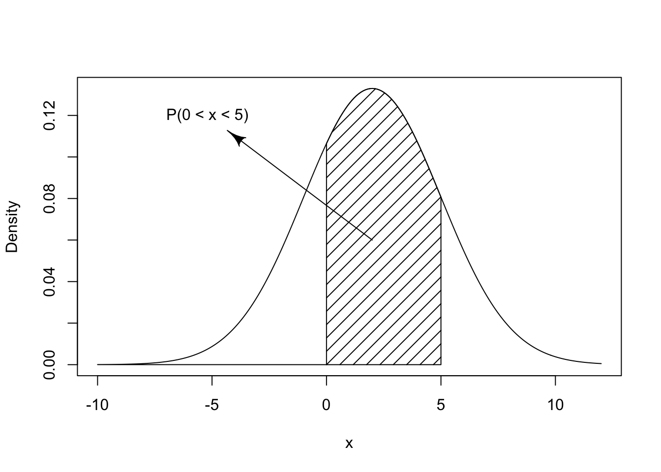
Consider, for example, \(X \sim \mathrm{Normal}(2,9)\text{.}\) The density of the distribution is presented in Figure 6.2.1. Observe that the distribution is symmetric about the expectation 2. The random variable is more likely to obtain its value in the vicinity of the expectation. Values much larger or much smaller than the expectation are substantially less likely.

The density of the Normal distribution can be computed with the aid of the function dnorm. The cumulative probability can be computed with the function pnorm. For illustrating the use of the latter function, assume that \(X \sim \mathrm{Normal}(2,9)\text{.}\) Say one is interested in the computation of the probability \(P(0 < X \leq 5)\) that the random variable obtains a value that belongs to the interval \((0,5]\text{.}\) The required probability is indicated by the marked area in Figure 6.2.1. This area can be computed as the difference between the probability \(P(X \leq 5)\text{,}\) the area to the left of 5, and the probability \(P(X \leq 0)\text{,}\) the area to the left of 0:

pnorm(5,2,3) - pnorm(0,2,3)

## [1] 0.5888522

The difference is the indicated area that corresponds to the probability of being inside the interval, which turns out to be approximately equal to 0.589. Notice that the expectation \(\mu\) of the Normal distribution is entered as the second argument to the function. The third argument to the function is the standard deviation, i.e. the square root of the variance. In this example, the standard deviation is \(\sqrt{9}=3\text{.}\)

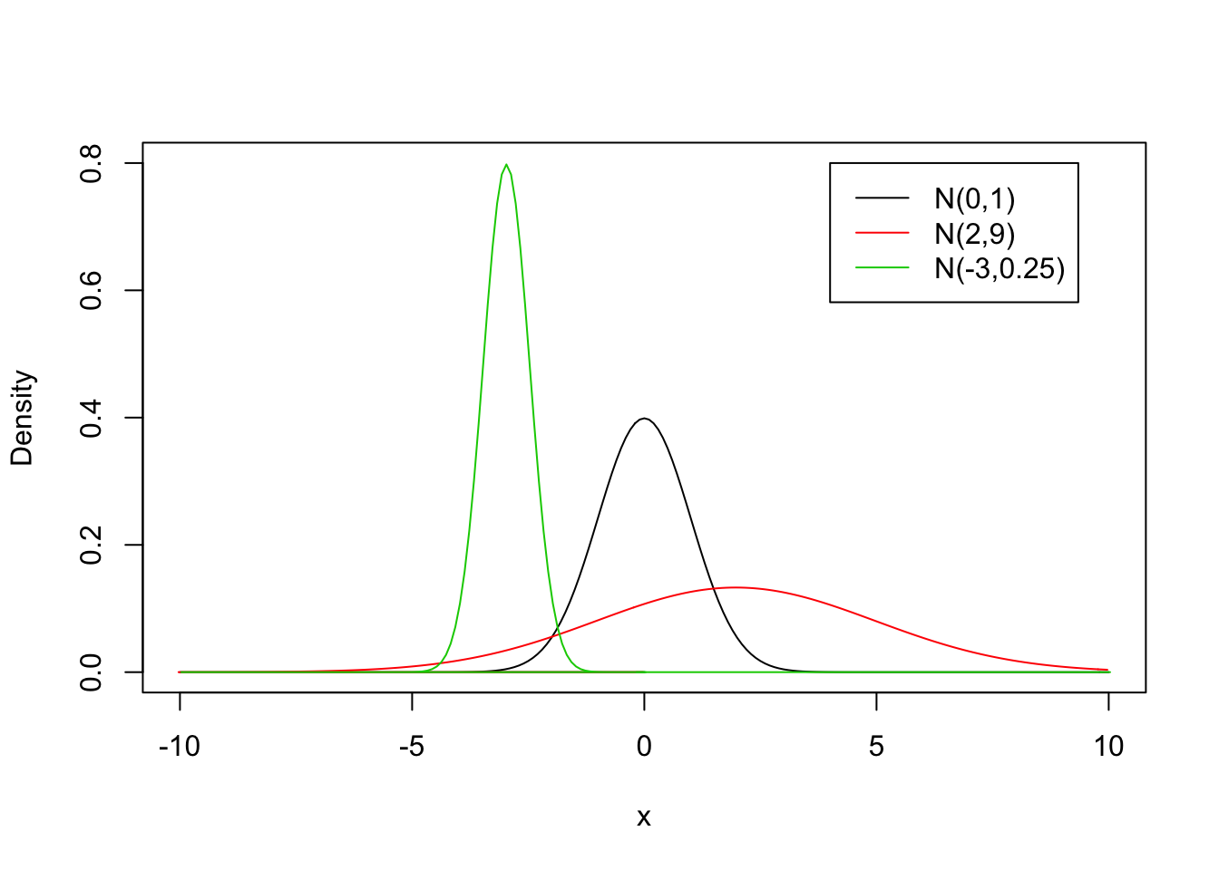
Figure 6.2.2 displays the densities of the Normal distribution for the combinations \(\mu= 0\text{,}\) \(\sigma^2 = 1\) (the red line); \(\mu = 2\text{,}\) \(\sigma^2 = 9\) (the black line); and \(\mu = -3\text{,}\) \(\sigma^2 = 1/4\) (the green line). Observe that the smaller the variance the more concentrated is the distribution of the random variable about the expectation.

The standard Normal distribution is a Normal distribution of standardized values, which are called \(z\)-scores. A \(z\)-score is the original measurement measured in units of the standard deviation from the expectation. For example, if the expectation of a Normal distribution is 2 and the standard deviation is \(3 = \sqrt{9}\text{,}\) then the value of 0 is 2/3 standard deviations smaller than (or to the left of) the expectation. Hence, the \(z\)-score of the value 0 is -2/3. The calculation of the \(z\)-score emerges from the equation:

The \(z\)-score is obtained by solving the equation

In a similar way, the \(z\)-score of the value \(x = 5\) is equal to 1, following the solution of the equation \(5 = 2 + z\cdot 3\text{,}\) which leads to \(z = (5-2)/3 = 1\text{.}\)

The standard Normal distribution is the distribution of a standardized Normal measurement. The expectation for the standard Normal distribution is 0 and the variance is 1. When \(X \sim N(\mu,\sigma^2)\) has a Normal distribution with expectation \(\mu\) and variance \(\sigma^2\) then the transformed random variable \(Z = (X-\mu)/\sigma\) produces the standard Normal distribution \(Z\sim N(0,1)\text{.}\) The transformation corresponds to the reexpression of the original measurement in terms of a new “zero” and a new unit of measurement. The new “zero” is the expectation of the original measurement and the new unit is the standard deviation of the original measurement.

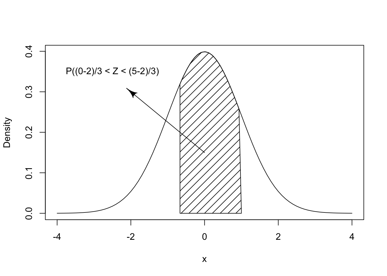
Computation of probabilities associated with a Normal random variable \(X\) can be carried out with the aid of the standard Normal distribution. For example, consider the computation of the probability \(P(0 < X \leq 5)\) for \(X \sim N(2, 9)\text{,}\) that has expectation \(\mu=2\) and standard deviation \(\sigma = 3\text{.}\) Consider \(X\)’s standardized values: \(Z = (X-2)/3\text{.}\) The boundaries of the interval \([0,5]\text{,}\) namely \(0\) and \(5\text{,}\) have standardized \(z\)-scores of \((0-2)/3=-2/3\) and \((5-2)/3 =1\text{,}\) respectively. Clearly, the original measurement \(X\) falls between the original boundaries (\(0 < X \leq 5\)) if, and only if, the standardized measurement \(Z\) falls between the standardized boundaries (\(-2/3 < Z \leq 1\)). Therefore, the probability that \(X\) obtains a value in the range \([0,5]\) is equal to the probability that \(Z\) obtains a value in the range \([-2/3,1]\text{.}\)

The function pnorm was used in the previous subsection in order to compute that probability that \(X\) obtains values between 0 and 5. The computation produced the probability 0.5888522. We can repeat the computation by the application of the same function to the standardized values:

pnorm((5-2)/3) - pnorm((0-2)/3)

## [1] 0.5888522

The value that is being computed, the area under the graph for the standard Normal distribution, is presented in Figure 6.2.5. Recall that 3 arguments were specified in the previous application of the function pnorm: the \(x\) value, the expectation, and the standard deviation. In the given application we did not specify the last two arguments, only the first one. (Notice that the output of the expression (5-2)/3 is a single number and, likewise, the output of the expression (0-2)/3 is also a single number.)

Most R functions have many arguments that enable flexible application in a wide range of settings. For convenience, however, default values are set to most of these arguments. These default values are used unless an alternative value for the argument is set when the function is called. The default value of the second argument of the function pnorm that specifies the expectation is mean=0, and the default value of the third argument that specifies the standard deviation is sd=1. Therefore, if no other value is set for these arguments the function computes the cumulative distribution function of the standard Normal distribution.

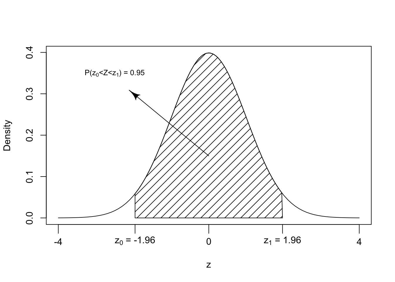
Consider the issue of determining the range that contains 95% of the probability for a Normal random variable. We start with the standard Normal distribution. Consult Figure 6.2.6. The figure displays the standard Normal distribution with the central region shaded. The area of the shaded region is 0.95.

We may find the \(z\)-values of the boundaries of the region, denoted in the figure as \(z_0\) and \(z_1\) by the investigation of the cumulative distribution function. Indeed, in order to have 95% of the distribution in the central region one should leave out 2.5% of the distribution in each of the two tails. That is, 0.025 should be the area of the unshaded region to the right of \(z_1\) and, likewise, 0.025 should be the area of the unshaded region to the left of \(z_0\text{.}\) In other words, the cumulative probability up to \(z_0\) should be 0.025 and the cumulative distribution up to \(z_1\) should be 0.975.

In general, given a random variable \(X\) and given a percent \(p\text{,}\) the \(x\) value with the property that the cumulative distribution up to \(x\) is equal to the probability \(p\) is called the \(p\)-percentile of the distribution. Here we seek the 2.5%-percentile and the 97.5%-percentile of the standard Normal distribution.

The percentiles of the Normal distribution are computed by the function qnorm. The first argument to the function is a probability (or a sequence of probabilities), the second and third arguments are the expectation and the standard deviations of the normal distribution. The default values to these arguments are set to 0 and 1, respectively. Hence if these arguments are not provided the function computes the percentiles of the standard Normal distribution. Let us apply the function in order to compute \(z_1\) and \(z_0\text{:}\)

qnorm(0.975)
qnorm(0.025)

## [1] 1.959964
## [1] -1.959964

Observe that \(z_1\) is practically equal to 1.96 and \(z_0 = -1.96 = -z_1\text{.}\) The fact that \(z_0\) is the negative of \(z_1\) results from the symmetry of the standard Normal distribution about 0. As a conclusion we get that for the standard Normal distribution 95% of the probability is concentrated in the range \([-1.96, 1.96]\text{.}\)

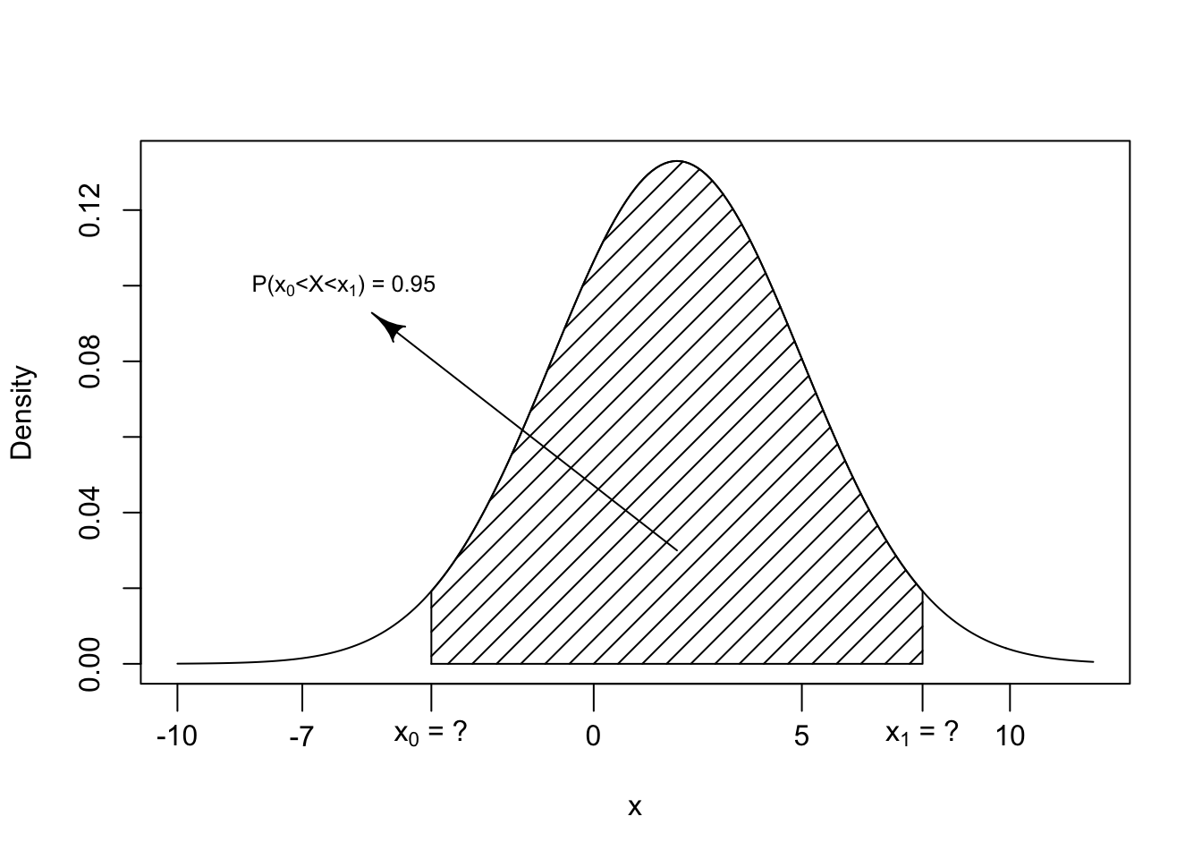
The problem of determining the central range that contains 95% of the distribution can be addressed in the context of the original measurement \(X\) (See Figure 6.2.7). We seek in this case an interval centered at the expectation 2, which is the center of the distribution of \(X\text{,}\) unlike 0 which was the center of the standardized values \(Z\text{.}\) One way of solving the problem is via the application of the function qnorm with the appropriate values for the expectation and the standard deviation:

qnorm(0.975,2,3)
qnorm(0.025,2,3)

## [1] 7.879892
## [1] -3.879892

Hence, we get that \(x_0 = -3.88\) has the property that the total probability to its left is 0.025 and \(x_1 = 7.88\) has the property that the total probability to its right is 0.025. The total probability in the range \([-3.88, 7.88]\) is 0.95.

An alternative approach for obtaining the given interval exploits the interval that was obtained for the standardized values. An interval \([-1.96,1.96]\) of standardized \(z\)-values corresponds to an interval \([2 - 1.96 \cdot 3, 2 + 1.96\cdot 3]\) of the original \(x\)-values:

2 + qnorm(0.975)*3
2 + qnorm(0.025)*3

## [1] 7.879892
## [1] -3.879892

Hence, we again produce the interval \([-3.88,7.88]\text{,}\) the interval that was obtained before as the central interval that contains 95% of the distribution of the \(\mathrm{Normal}(2,9)\) random variable.

In general, if \(X \sim N(\mu,\sigma^2)\) is a Normal random variable then the interval \([\mu - 1.96 \cdot \sigma, \mu + 1.96 \cdot \sigma]\) contains 95% of the distribution of the random variable. Frequently one uses the notation \(\mu \pm 1.96 \cdot \sigma\) to describe such an interval.

Consider, next, the computation of the interquartile range in the Normal distribution. Recall that the interquartile range is the length of the central interval that contains 50% of the distribution. This interval starts at the first quartile (Q1), the value that splits the distribution so that 25% of the distribution is to the left of the value and 75% is to the right of it. The interval ends at the third quartile (Q3) where 75% of the distribution is to the left and 25% is to the right.

For the standard Normal the third and first quartiles can be computed with the aid of the function qnorm:

qnorm(0.75)
qnorm(0.25)

## [1] 0.6744898
## [1] -0.6744898

Observe that for the standard Normal distribution one has that 75% of the distribution is to the left of the value 0.6744898, which is the third quartile of this distribution. Likewise, 25% of the standard Normal distribution are to the left of the value -0.6744898, which is the first quartile. The interquartile range is the length of the interval between the third and the first quartiles. In the case of the standard Normal distribution this length is equal to \(0.6744898 - (-0.6744898) = 1.348980\text{.}\)

In Chapter 3 we considered box plots as a means for the graphical display of numerical data. The box plot includes a vertical rectangle that initiates at the first quartile and ends at the third quartile, with the median marked within the box. The rectangle contains 50% of the data. Whiskers extend from the ends of this rectangle to the smallest and to the largest data values that are not outliers. Outliers are values that lie outside of the normal range of the data. Outliers are identified as values that are more than 1.5 times the interquartile range away from the ends of the central rectangle. Hence, a value is an outlier if it is larger than the third quartile plus 1.5 times the interquartile range or if it is less than the first quartile minus 1.5 times the interquartile range.

How likely is it to obtain an outlier value when the measurement has the standard Normal distribution? We obtained that the third quartile of the standard Normal distribution is equal to 0.6744898 and the first quartile is minus this value. The interquartile range is the difference between the third and first quartiles. The upper and lower thresholds for the defining outliers are:

qnorm(0.75) + 1.5*(qnorm(0.75)-qnorm(0.25))
qnorm(0.25) - 1.5*(qnorm(0.75)-qnorm(0.25))

## [1] 2.697959
## [1] -2.697959

Hence, a value larger than 2.697959 or smaller than -2.697959 would be identified as an outlier.

The probability of being less than the upper threshold 2.697959 in the standard Normal distribution is computed with the expression pnorm(2.697959). The probability of being above the threshold is 1 minus that probability, which is the outcome of the expression 1-pnorm(2.697959).

By the symmetry of the standard Normal distribution we get that the probability of being below the lower threshold -2.697959 is equal to the probability of being above the upper threshold. Consequently, the probability of obtaining an outlier is equal to twice the probability of being above the upper threshold:

2*(1-pnorm(2.697959))

## [1] 0.006976603

We get that for the standard Normal distribution the probability of an outlier is approximately 0.7%.