As an application of the Binomial distribution consider a pre-election poll. A candidate is running for office and is interested in knowing the percentage of support in the general population in its candidacy. Denote the probability of support by \(p\text{.}\) In order to estimate the percentage a sample of size 300 is selected from the population. Let \(X\) be the count of supporters in the sample. A natural model for the distribution of \(X\) is the \(\mathrm{Binomial}(300,p)\) distribution, since each subject in the sample may be a supporter (“Success") or may not be a supporter (“Failure"). The probability that a subject supports the candidate is \(p\) and there are \(n=300\) subjects in the sample.
Section 5.2 Discrete Random Variables
In the previous chapter we introduced the notion of a random variable. A random variable corresponds to the outcome of an observation or a measurement prior to the actual making of the measurement. In this context one can talk of all the values that the measurement may potentially obtain. This collection of values is called the sample space. To each value in the sample space one may associate the probability of obtaining this particular value. Probabilities are like relative frequencies. All probabilities are positive and the sum of the probabilities that are associated with all the values in the sample space is equal to one.
A random variable is defined by the identification of its sample space and the probabilities that are associated with the values in the sample space. For each type of random variable we will identify first the sample space — the values it may obtain — and then describe the probabilities of the values. Examples of situations in which each type of random variable may serve as a model of a measurement will be provided. The
R system provides functions for the computation of probabilities associated with specific types of random variables. We will use these functions in this and in proceeding chapters in order to carry out computations associated with the random variables and in order to plot their distributions.
The distribution of a random variable, just like the distribution of data, can be characterized using numerical summaries. For the latter we used summaries such as the mean and the sample variance and standard deviation. The mean is used to describe the central location of the distribution and the variance and standard deviation are used to characterize the total spread. Parallel summaries are used for random variable. In the case of a random variable the name expectation is used for the central location of the distribution and the variance and the standard deviation (the square root of the variation) are used to summarize the spread. In all the examples of random variables we will identify the expectation and the variance (and, thereby, also the standard deviation).
Random variables are used as probabilistic models of measurements. Theoretical considerations are used in many cases in order to define random variables and their distribution. A random variable for which the values in the sample space are separated from each other, say the values are integers, is called a discrete random variable. In this section we introduce two important integer-valued random variables: The Binomial and the Poisson random variables. These random variables may emerge as models in contexts where the measurement involves counting the number of occurrences of some phenomena.
Many other models, apart from the Binomial and Poisson, exist for discrete random variables. An example of such model, the Negative-Binomial model, will be considered in Section 5.4. Depending on the specific context that involves measurements with discrete values, one may select the Binomial, the Poisson, or one of these other models to serve as a theoretical approximation of the distribution of the measurement.
Subsection 5.2.1 The Binomial Random Variable
The Binomial random variable is used in settings in which a trial that has two possible outcomes is repeated several times. Let us designate one of the outcomes as “Success" and the other as “Failure". Assume that the probability of success in each trial is given by some number \(p\) that is larger than 0 and smaller than 1. Given a number \(n\) of repeats of the trial and given the probability of success, the actual number of trials that will produce “Success" as their outcome is a random variable. We call such random variable Binomial. The fact that a random variable \(X\) has such a distribution is marked by the expression: “\(X \sim \mathrm{Binomial}(n,p)\)".
As an example consider tossing 10 coins. Designate “Head" as success and “Tail" as failure. For fair coins the probability of “Head" is \(1/2\text{.}\) Consequently, if \(X\) is the total number of “Heads" then \(X \sim \mathrm{Binomial}(10,0.5)\text{,}\) where \(n=10\) is the number of trials and \(p=0.5\) is the probability of success in each trial.
It may happen that all 10 coins turn up “Tail". In this case \(X\) is equal to 0. It may also be the case that one of the coins turns up “Head" and the others turn up “Tail". The random variable \(X\) will obtain the value 1 in such a case. Likewise, for any integer between 0 and 10 it may be the case that the number of “Heads" that turn up is equal to that integer with the other coins turning up “Tail". Hence, the sample space of \(X\) is the set of integers \(\{0, 1, 2, \ldots, 10\}\text{.}\) The probability of each outcome may be computed by an appropriate mathematical formula that will not be discussed here.
1
If \(X\sim \mathrm{Binomial}(n,p)\) then \(\Prob(X = x) = {n \choose x} p^x (1-p)^{n-x}\text{,}\) for \(x = 0, 1, \ldots, n\text{.}\)
The probabilities of the various possible values of a Binomial random variable may be computed with the aid of the
R function “dbinom" (that uses the mathematical formula for the computation). The input to this function is a sequence of values, the value of \(n\text{,}\) and the value of \(p\text{.}\) The output is the sequence of probabilities associated with each of the values in the first input.
For example, let us use the function in order to compute the probability that the given Binomial obtains an odd value. A sequence that contains the odd values in the Binomial sample space can be created with the expression “
c(1,3,5,7,9)". This sequence can serve as the input in the first argument of the function “dbinom". The other arguments are “10" and “0.5", respectively:
dbinom(c(1,3,5,7,9),10,0.5)
## [1] 0.009765625 0.117187500 0.246093750 0.117187500 0.009765625
Observe that the output of the function is a sequence of the same length as the first argument. This output contains the Binomial probabilities of the values in the first argument. In order to obtain the probability of the event \(\{\mbox{X is odd}\}\) we should sum up these probabilities, which we can do by applying the function “
sum" to the output of the function that computes the Binomial probabilities:
sum(dbinom(c(1,3,5,7,9),10,0.5))
## [1] 0.5
Observe that the probability of obtaining an odd value in this specific case is equal to one half.
Another example is to compute all the probabilities of all the potential values of a \(\mathrm{Binomial}(10,0.5)\) random variable:
x <- 0:10
dbinom(x,10,0.5)
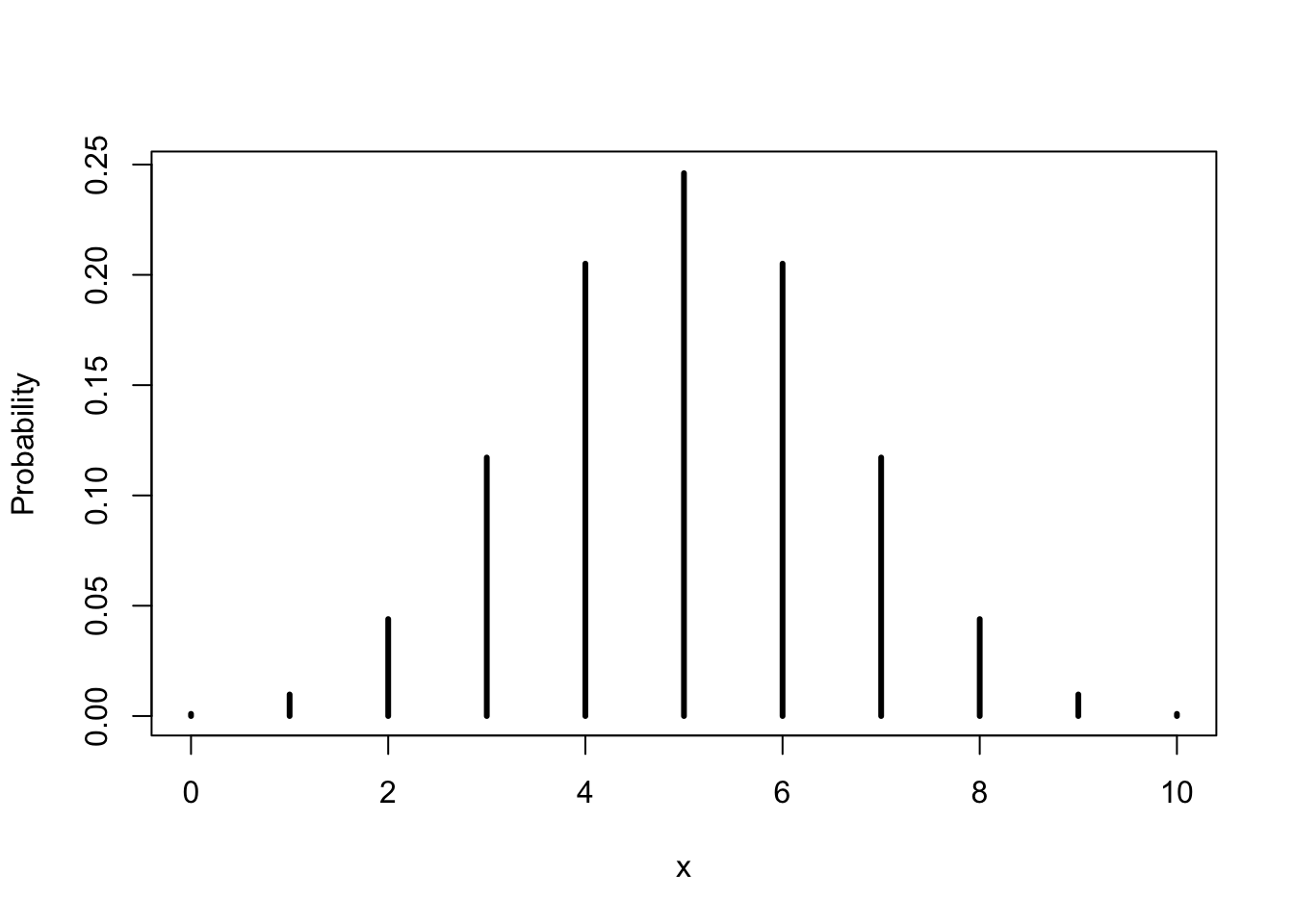
##  [1] 0.0009765625 0.0097656250 0.0439453125 0.1171875000 0.2050781250
##  [6] 0.2460937500 0.2050781250 0.1171875000 0.0439453125 0.0097656250
## [11] 0.0009765625
The expression “
start.value:end.value" produces a sequence of numbers that initiate with the number “start.value" and proceeds in jumps of size one until reaching the number “end.value". In this example, “0:10" produces the sequence of integers between 0 and 10, which is the sample space of the current Binomial example. Entering this sequence as the first argument to the function “dbinom" produces the probabilities of all the values in the sample space.
One may display the distribution of a discrete random variable with a bar plot similar to the one used to describe the distribution of data. In this plot a vertical bar representing the probability is placed above each value of the sample space. The height of the bar is equal to the probability. A bar plot of the \(\mathrm{Binomial}(10,0.5)\) distribution is provided in Figure 5.2.1.
Another useful function is “
pbinom", which produces the cumulative probability of the Binomial:
pbinom(x,10,0.5)
cumsum(dbinom(x,10,0.5))
##  [1] 0.0009765625 0.0107421875 0.0546875000 0.1718750000 0.3769531250
##  [6] 0.6230468750 0.8281250000 0.9453125000 0.9892578125 0.9990234375
## [11] 1.0000000000
##  [1] 0.0009765625 0.0107421875 0.0546875000 0.1718750000 0.3769531250
##  [6] 0.6230468750 0.8281250000 0.9453125000 0.9892578125 0.9990234375
## [11] 1.0000000000
The output of the function “
pbinom" is the cumulative probability \(\Prob(X \leq x)\) that the random variable is less than or equal to the input value. Observe that this cumulative probability is obtained by summing all the probabilities associated with values that are less than or equal to the input value. Specifically, the cumulative probability at \(x=3\) is obtained by the summation of the probabilities at \(x=0\text{,}\) \(x=1\text{,}\) \(x=2\text{,}\) and \(x=3\text{:}\)
\begin{equation*}
\Prob(X \leq 3) = 0.0009765625 + 0.009765625 + 0.0439453125 + 0.1171875 = 0.171875
\end{equation*}
The numbers in the sum are the first 4 values from the output of the function “
dbinom(x,10,0.5)", which computes the probabilities of the values of the sample space.In principle, the expectation of the Binomial random variable, like the expectation of any other (discrete) random variable is obtained from the application of the general formulae:
\begin{equation*}
\Expec(X) = \sum_x \big(x \times \Prob(X = x)\big)\;,\quad \Var(X) = \sum_x\big( (x-\Expec(X))^2 \times \Prob(x)\big)\;.
\end{equation*}
However, in the specific case of the Binomial random variable, in which the probability \(\Prob(X = x)\) obeys the specific mathematical formula of the Binomial distribution, the expectation and the variance reduce to the specific formulae:
\begin{equation*}
\Expec(X) = n p\;,\quad \Var(X) = n p(1-p)\;.
\end{equation*}
Hence, the expectation is the product of the number of trials \(n\) with the probability of success in each trial \(p\text{.}\) In the variance the number of trials is multiplied by the product of a probability of success (\(p\)) with the probability of a failure (\(1-p\)).
As illustration, let us compute for the given example the expectation and the variance according to the general formulae for the computation of the expectation and variance in random variables and compare the outcome to the specific formulae for the expectation and variance in the Binomial distribution:
X.val <- 0:10
P.val <- dbinom(X.val,10,0.5)
EX <- sum(X.val*P.val)
EX
sum((X.val-EX)^2*P.val)
## [1] 5
## [1] 2.5
This agrees with the specific formulae for Binomial variables, since \(10 \times 0.5 = 5\) and \(10 \times 0.5 \times(1-0.5) = 2.5\text{.}\)
Recall that the general formula for the computation of the expectation calls for the multiplication of each value in the sample space with the probability of that value, followed by the summation of all the products. The object “
X.val" contains all the values of the random variable and the object “P.val" contains the probabilities of these values. Hence, the expression “X.val*P.val" produces the product of each value of the random variable times the probability of that value. Summation of these products with the function “sum" gives the expectation, which is saved in an object that is called “EX".
The general formula for the computation of the variance of a random variable involves the product of the squared deviation associated with each value with the probability of that value, followed by the summation of all products. The expression “
(X.val-EX)^ 2" produces the sequence of squared deviations from the expectation for all the values of the random variable. Summation of the product of these squared deviations with the probabilities of the values (the outcome of “(X.val-EX)^2*P.val") gives the variance.
When the value of \(p\) changes (without changing the number of trials \(n\)) then the probabilities that are assigned to each of the values of the sample space of the Binomial random variable change, but the sample space itself does not. For example, consider rolling a die 10 times and counting the number of times that the face 3 was obtained. Having the face 3 turning up is a “Success". The probability \(p\) of a success in this example is 1/6, since the given face is one out of 6 equally likely faces. The resulting random variable that counts the total number of success in 10 trials has a \(\mathrm{Binomial}(10,1/6)\) distribution. The sample space is yet again equal to the set of integers \(\{0,1, \ldots,10\}\text{.}\) However, the probabilities of values are different. These probabilities can again be computed with the aid of the function “
dbinom":
dbinom(x,10,1/6)
##  [1] 1.615056e-01 3.230112e-01 2.907100e-01 1.550454e-01 5.426588e-02
##  [6] 1.302381e-02 2.170635e-03 2.480726e-04 1.860544e-05 8.269086e-07
## [11] 1.653817e-08
In this case smaller values of the random variable are assigned higher probabilities and larger values are assigned lower probabilities.
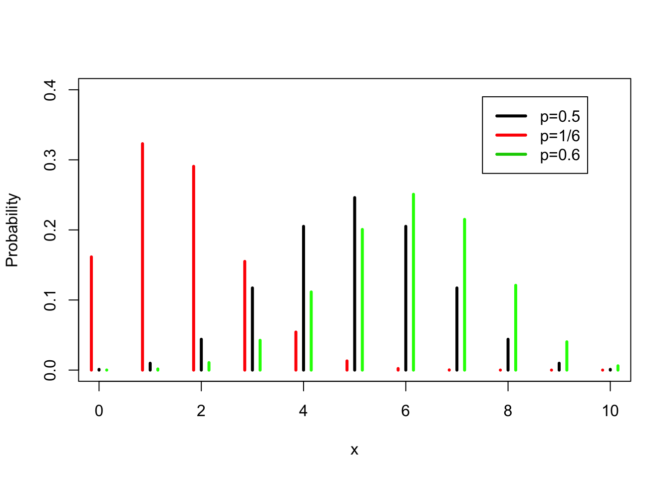
In Figure 5.2.2 the probabilities for \(\mathrm{Binomial}(10,1/6)\text{,}\) the \(\mathrm{Binomial}(10,1/2)\text{,}\) and the \(\mathrm{Binomial}(10,0.6)\) distributions are plotted side by side. In all these 3 distributions the sample space is the same, the integers between 0 and 10. However, the probabilities of the different values differ. (Note that all bars should be placed on top of the integers. For clarity of the presentation, the bars associated with the \(\mathrm{Binomial}(10,1/6)\) are shifted slightly to the left and the bars associated with the \(\mathrm{Binomial}(10,0.6)\) are shifted slightly to the right.)
The expectation of the \(\mathrm{Binomial}(10,0.5)\) distribution is equal to \(10 \times 0.5 = 5\text{.}\) Compare this to the expectation of the \(\mathrm{Binomial}(10,1/6)\) distribution, which is \(10 \times (1/6) = 1.666667\) and to the expectation of the \(\mathrm{Binomial}(10,0.6)\) distribution which equals \(10 \times 0.6 = 6\text{.}\)
The variance of the \(\mathrm{Binomial}(10,0.5)\) distribution is \(10 \times 0.5 \times 0.5 = 2.5\text{.}\) The variance when \(p=1/6\) is \(10 \times (1/6) \times (5/6) = 1.388889\) and the variance when \(p=0.6\) is \(10 \times 0.6 \times 0.4 = 2.4\text{.}\)
Example 5.2.3.
Example 5.2.4.
As another example consider the procedure for quality control that is described in Discussion Forum of Chapter 4. According to the procedure 20 items are tested and the number of faulty items is recorded. If \(p\) is the probability that an item is identified as faulty then the distribution of the total number of faulty items may be modeled by the \(\mathrm{Binomial}(20,p)\) distribution.
In both examples one may be interested in making statements on the probability \(p\) based on the sample. Statistical inference relates the actual count obtained in the sample to the theoretical Binomial distribution in order to make such statements.
Subsection 5.2.2 The Poisson Random Variable
The Poisson distribution is used as an approximation of the total number of occurrences of rare events. Consider, for example, the Binomial setting that involves \(n\) trials with \(p\) as the probability of success of each trial. Then, if \(p\) is small but \(n\) is large then the number of successes \(X\) has, approximately, the Poisson distribution.
The sample space of the Poisson random variable is the unbounded collection of integers: \(\{0,1,2, \ldots\}\text{.}\) Any integer value is assigned a positive probability. Hence, the Poisson random variable is a convenient model when the maximal number of occurrences of the events in a-priori unknown or is very large. For example, one may use the Poisson distribution to model the number of phone calls that enter a switchboard in a given interval of time or the number of malfunctioning components in a shipment of some product.
The Binomial distribution was specified by the number of trials \(n\) and probability of success in each trial \(p\text{.}\) The Poisson distribution is specified by its expectation, which we denote by \(\lambda\text{.}\) The expression “\(X \sim \mathrm{Poisson}(\lambda)\)" states that the random variable \(X\) has a Poisson distribution with expectation \(\Expec(X) = \lambda\text{.}\) The function “
2
If \(X \sim \mathrm{Poisson}(\lambda)\) then \(\Prob(X=x) = e^{-\lambda}\lambda^x/x!\text{,}\) for \(x=0,1,2,\ldots\text{.}\)
dpois" computes the probability, according to the Poisson distribution, of values that are entered as the first argument to the function. The expectation of the distribution is entered in the second argument. The function “ppois" computes the cumulative probability. Consequently, we can compute the probabilities and the cumulative probabilities of the values between 0 and 10 for the \(\mathrm{Poisson}(2)\) distribution via:
x <- 0:10
dpois(x,2)
ppois(x,2)
##  [1] 1.353353e-01 2.706706e-01 2.706706e-01 1.804470e-01 9.022352e-02
##  [6] 3.608941e-02 1.202980e-02 3.437087e-03 8.592716e-04 1.909493e-04
## [11] 3.818985e-05
##  [1] 0.1353353 0.4060058 0.6766764 0.8571235 0.9473470 0.9834364 0.9954662
##  [8] 0.9989033 0.9997626 0.9999535 0.9999917
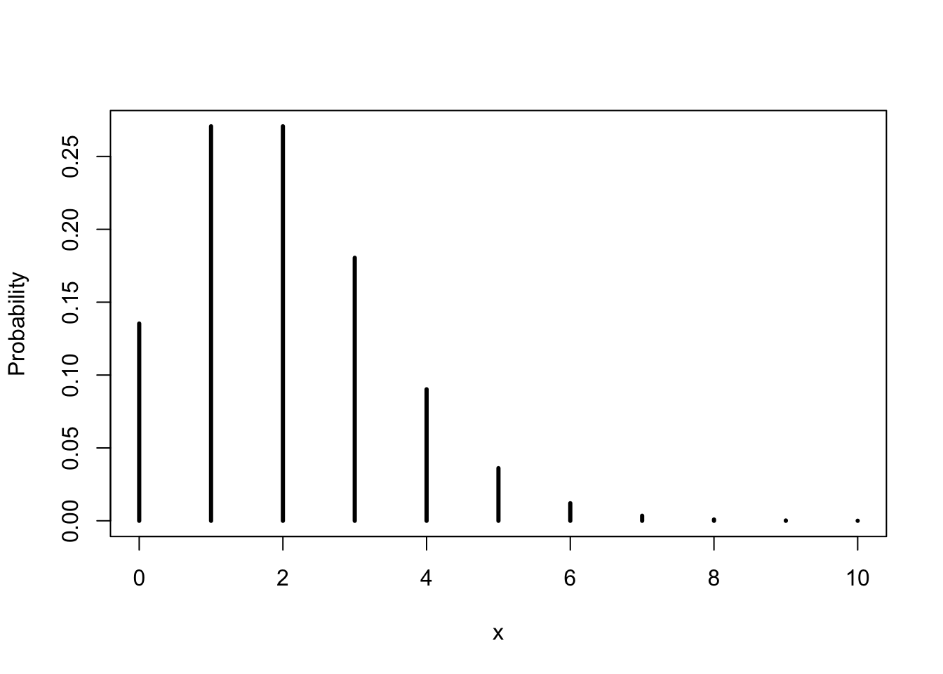
The probability function of the Poisson distribution with \(\lambda = 2\text{,}\) in the range between 0 and 10, is plotted in Figure 5.2.5. Observe that in this example probabilities of the values 8 and beyond are very small. As a matter of fact, the cumulative probability at \(x=7\) (the 8th value in the output of “
ppois(x,2)") is approximately 0.999, out of the total cumulative probability of 1.000, leaving a total probability of about 0.001 to be distributed among all the values larger than 7.
Let us compute the expectation of the given Poisson distribution:
X.val <- 0:10
P.val <- dpois(X.val,2)
sum(X.val*P.val)
## [1] 1.999907
Observe that the outcome is almost, but not quite, equal to \(2.00\text{,}\) which is the actual value of the expectation. The reason for the inaccuracy is the fact that we have based the computation in
R on the first 11 values of the distribution only, instead of the infinite sequence of values. A more accurate result may be obtained by the consideration of the first 101 values:
X.val <- 0:100
P.val <- dpois(X.val,2)
EX <- sum(X.val*P.val)
EX
sum((X.val-EX)^2*P.val)
## [1] 2
## [1] 2
In the last expression we have computed the variance of the Poisson distribution and obtained that it is equal to the expectation. This results can be validated mathematically. For the Poisson distribution it is always the case that the variance is equal to the expectation, namely to \(\lambda\text{:}\)
\begin{equation*}
\Expec(X) = \Var(X) = \lambda\;.
\end{equation*}
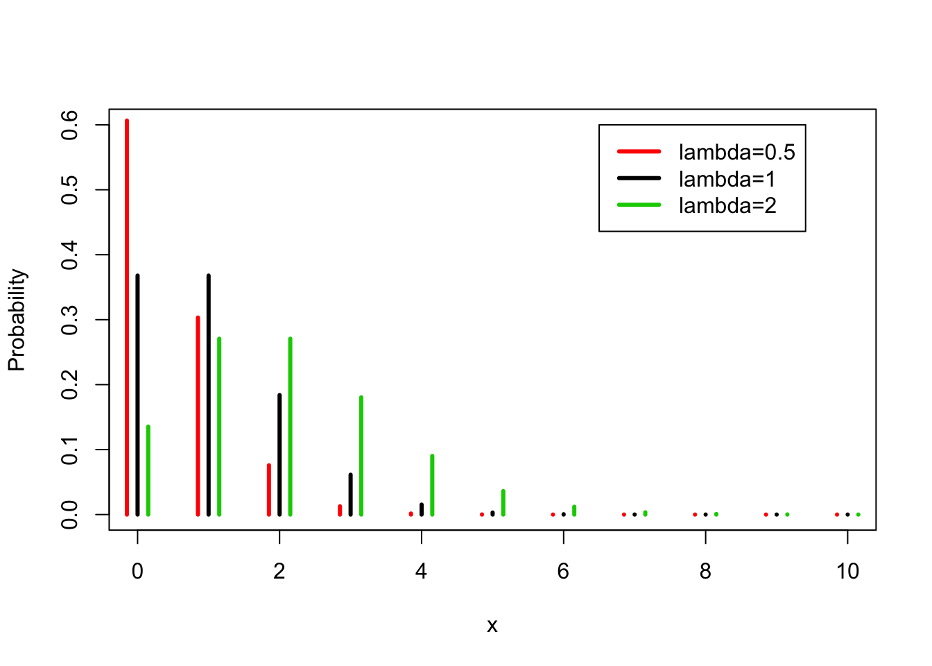
In Figure 5.2.6 you may find the probabilities of the Poisson distribution for \(\lambda = 0.5\text{,}\) \(\lambda = 1\) and \(\lambda = 2\text{.}\) Notice once more that the sample space is the same for all the Poisson distributions. What varies when we change the value of \(\lambda\) are the probabilities. Observe that as \(\lambda\) increases then probability of larger values increases as well.
Example 5.2.7.
A radio active element decays by the release of subatomic particles and energy. The decay activity is measured in terms of the number of decays per second in a unit mass. A typical model for the distribution of the number of decays is the Poisson distribution. Observe that the number of decays in a second is a integer and, in principle, it may obtain any integer value larger or equal to zero. The event of a radio active decay of an atom is a relatively rare event. Therefore, the Poisson model is likely to fit this phenomena.
3
The number of decays may also be considered in the \(\mathrm{Binomial}(n,p)\) setting. The number \(n\) is the total number of atoms in the unit mass and \(p\) is the probability that an atom decays within the given second. However, since \(n\) is very large and \(p\) is very small we get that the Poisson distribution is an appropriate model for the count.
Example 5.2.8.
Consider an overhead power line suspended between two utility poles. During rain, drops of water may hit the power line. The total number of drops that hit the line in a one minute period may be modeled by a Poisson random variable.

