In Example 5.2.8 we considered rain drops that hit an overhead power line suspended between two utility poles. The number of drops that hit the line can be modeled using the Poisson distribution. The position between the two poles where a rain drop hits the line can be modeled by the Uniform distribution. The rain drop can hit any position between the two utility poles. Hitting one position along the line is as likely as hitting any other position.
Section 5.3 Continuous Random Variables
Many types of measurements, such as height, weight, angle, temperature, etc., may in principle have a continuum of possible values. Continuous random variables are used to model uncertainty regarding future values of such measurements.
The main difference between discrete random variables, which is the type we examined thus far, and continuous random variable, that are added now to the list, is in the sample space, i.e., the collection of possible outcomes. The former type is used when the possible outcomes are separated from each other as the integers are. The latter type is used when the possible outcomes are the entire line of real numbers or when they form an interval (possibly an open ended one) of real numbers.
The difference between the two types of sample spaces implies differences in the way the distribution of the random variables is being described. For discrete random variables one may list the probability associated with each value in the sample space using a table, a formula, or a bar plot. For continuous random variables, on the other hand, probabilities are assigned to intervals of values, and not to specific values. Thence, densities are used in order to display the distribution.
Densities are similar to histograms, with areas under the plot corresponding to probabilities. We will provide a more detailed description of densities as we discuss the different examples of continuous random variables.
In continuous random variables integration replaces summation and the density replaces the probability in the computation of quantities such as the probability of an event, the expectation, and the variance.
Hence, if the expectation of a discrete random variable is given in the formula \(\Expec(X) = \sum_x \big(x \times \Prob(x)\big)\text{,}\) which involves the summation over all values of the product between the value and the probability of the value, then for continuous random variable the definition becomes:
\begin{equation*}
\Expec(X) = \int \big(x \times f(x)\big)dx\;,
\end{equation*}
where \(f(x)\) is the density of \(X\) at the value \(x\text{.}\) Therefore, in the expectation of a continuous random variable one multiplies the value by the density at the value. This product is then integrated over the sample space.
Likewise, the formula \(\Var(X) = \sum_x\big( (x-\Expec(X))^2 \times \Prob(x)\big)\) for the variance is replaced by:
\begin{equation*}
\Var(X) =\int\big((x-\Expec(X))^2 \times f(x) \big) dx\;.
\end{equation*}
Nonetheless, the intuitive interpretation of the expectation as the central value of the distribution that identifies the location and the interpretation of the standard deviation (the square root of the variance) as the summary of the total spread of the distribution is still valid.
In this section we will describe two types of continuous random variables: Uniform and Exponential. In the next chapter another example – the Normal distribution – will be introduced.
Subsection 5.3.1 The Uniform Random Variable
The Uniform distribution is used in order to model measurements that may have values in a given interval, with all values in this interval equally likely to occur.
For example, consider a random variable \(X\) with the Uniform distribution over the interval \([3,7]\text{,}\) denoted by “\(X \sim \mathrm{Uniform}(3,7)\)". The density function at given values may be computed with the aid of the function “
dunif". For instance let us compute the density of the \(\mathrm{Uniform}(3,7)\) distribution over the integers \(\{0, 1, \ldots, 10\}\text{:}\)
dunif(0:10,3,7)
## [1] 0.00 0.00 0.00 0.25 0.25 0.25 0.25 0.25 0.00 0.00 0.00
Notice that for the values 0, 1, and 2, and the values 8, 9 and 10 that are outside of the interval the density is equal to zero, indicating that such values cannot occur in the given distribution. The values of the density at integers inside the interval are positive and equal to each other. The density is not restricted to integer values. For example, at the point \(4.73\) we get that the density is positive and of the same height:
dunif(4.73,3,7)
## [1] 0.25
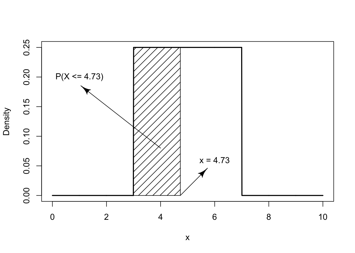
A plot of the \(\mathrm{Uniform}(3,7)\) density is given in Figure 5.3.1 in the form of a solid line. Observe that the density is positive over the interval \([3,7]\) where its height is 1/4. Area under the curve in the density corresponds to probability. Indeed, the fact that the total probability is one is reflected in the total area under the curve being equal to 1. Over the interval \([3,7]\) the density forms a rectangle. The base of the rectangle is the length of the interval \(7-3=4\text{.}\) The height of the rectangle is thus equal to 1/4 in order to produce a total area of \(4 \times (1/4) = 1\text{.}\)
The function “
punif" computes the cumulative probability of the uniform distribution. The probability \(\Prob(X \leq 4.73)\text{,}\) for \(X \sim \mathrm{Uniform}(3,7)\text{,}\) is given by:
punif(4.73,3,7)
## [1] 0.4325
This probability corresponds to the marked area to the left of the point \(x = 4.73\) in Figure 5.3.1. This area of the marked rectangle is equal to the length of the base 4.73 - 3 = 1.73, times the height of the rectangle 1/(7-3) = 1/4. Indeed:
(4.73-3)/(7-3)
## [1] 0.4325
is the area of the marked rectangle and is equal to the probability.
Let us use
R in order to plot the density and the cumulative probability functions of the Uniform distribution. We produce first a large number of points in the region we want to plot. The points are produced with aid of the function “seq". The output of this function is a sequence with equally spaced values. The starting value of the sequence is the first argument in the input of the function and the last value is the second argument in the input. The argument “length=1000" sets the length of the sequence, 1,000 values in this case:
x <- seq(0,10,length=1000)
den <- dunif(x,3,7)
plot(x,den)

The object “
den" is a sequence of length 1,000 that contains the density of the \(\mathrm{Uniform}(3,7)\) evaluated over the values of “x". When we apply the function “plot" to the two sequences we get a scatter plot of the 1,000 points.
A scatter plot is a plot of points. Each point in the scatter plot is identify by its horizontal location on the plot (its “\(x\)" value) and by its vertical location on the plot (its \(y\) value). The horizontal value of each point in the plot is determined by the first argument to the function “
plot" and the vertical value is determined by the second argument. For example, the first value in the sequence “x" is 0. The value of the Uniform density at this point is 0. Hence, the first value of the sequence “den" is also 0. A point that corresponds to these values is produced in the plot. The horizontal value of the point is 0 and the vertical value is 0. In a similar way the other 999 points are plotted. The last point to be plotted has a horizontal value of 10 and a vertical value of 0.
The number of points that are plotted is large and they overlap each other in the graph and thus produce an impression of a continuum. In order to obtain nicer looking plots we may choose to connect the points to each other with segments and use smaller points. This may be achieved by the addition of the argument “
type=l", with the letter l for line, to the plotting function:
plot(x,den,type="l")

The cumulative probability of the \(\mathrm{Uniform}(3,7)\) is produced by the code:
cdf <- punif(x,3,7)
plot(x,cdf,type="l")

One can think of the density of the Uniform as an histogram. The expectation of a Uniform random variable is the middle point of it’s histogram. Hence, if \(X \sim \mathrm{Uniform}(a,b)\) then:
1
If \(X \sim \mathrm{Uniform}(a,b)\) then the density is \(f(x) = 1/(b-a)\text{,}\) for \(a \leq x \leq b\text{,}\) and it is equal to 0 for other values of \(x\text{.}\)
\begin{equation*}
\Expec(X) = \frac{a+b}{2}\;.
\end{equation*}
For the \(X \sim \mathrm{Uniform}(3,7)\) distribution the expectation is \(\Expec(X)= (3+7)/2 = 5\text{.}\) Observe that 5 is the center of the Uniform density in Plot Figure 5.3.1.
It can be shown that the variance of the \(\mathrm{Uniform}(a,b)\) is equal to
\begin{equation*}
\Var(X) = \frac{(b-a)^2}{12}\;,
\end{equation*}
with the standard deviation being the square root of this value. Specifically, for \(X \sim \mathrm{Uniform}(3,7)\) we get that \(\Var(X) = (7-3)^2/12 = 1.333333\text{.}\) The standard deviation is equal to \(\sqrt{1.333333} = 1.154701\text{.}\)
Example 5.3.5.
Example 5.3.6.
Meiosis is the process in which a diploid cell that contains two copies of the genetic material produces an haploid cell with only one copy (sperms or eggs, depending on the sex). The resulting molecule of genetic material is linear molecule (chromosome) that is composed of consecutive segments: a segment that originated from one of the two copies followed by a segment from the other copy and vice versa. The border points between segments are called points of crossover. The Haldane model for crossovers states that the position of a crossover between two given loci on the chromosome corresponds to the Uniform distribution and the total number of crossovers between these two loci corresponds to the Poisson distribution.
Subsection 5.3.2 The Exponential Random Variable
The Exponential distribution is frequently used to model times between events. For example, times between incoming phone calls, the time until a component becomes malfunction, etc. We denote the Exponential distribution via “\(X \sim \mathrm{Exponential}(\lambda)\)", where \(\lambda\) is a parameter that characterizes the distribution and is called the rate of the distribution. The overlap between the parameter used to characterize the Exponential distribution and the one used for the Poisson distribution is deliberate. The two distributions are tightly interconnected. As a matter of fact, it can be shown that if the distribution between occurrences of a phenomena has the Exponential distribution with rate \(\lambda\) then the total number of the occurrences of the phenomena within a unit interval of time has a \(\mathrm{Poisson}(\lambda)\) distribution.
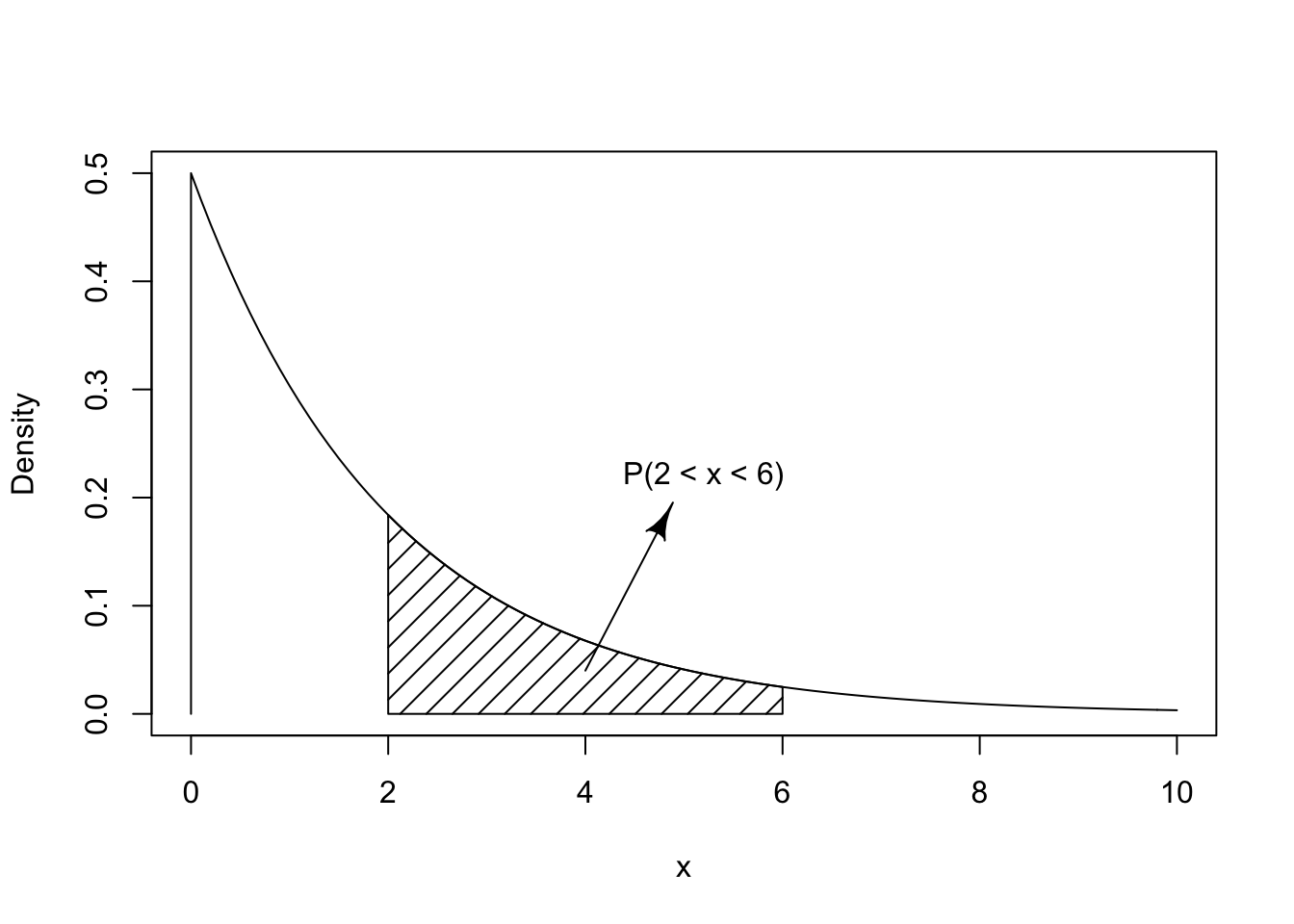
The sample space of an Exponential random variable contains all non-negative numbers. Consider, for example, \(X \sim \mathrm{Exponential}(0.5)\text{.}\) The density of the distribution in the range between 0 and 10 is presented in Figure 5.3.7. Observe that in the Exponential distribution smaller values are more likely to occur in comparison to larger values. This is indicated by the density being larger at the vicinity of 0. The density of the exponential distribution given in the plot is positive, but hardly so, for values larger than 10.
The density of the Exponential distribution can be computed with the aid of the function “. The cumulative probability can be computed with the function “
dexp"2
If \(X \sim \mathrm{Exponential}(\lambda)\) then the density is \(f(x) =\lambda e^{-\lambda x}\text{,}\) for \(0 \leq x\text{,}\) and it is equal to 0 for \(x < 0\text{.}\)
pexp". For illustration, assume \(X \sim \mathrm{Exponential}(0.5)\text{.}\) Say one is interested in the computation of the probability \(\Prob(2 < X \leq 6)\) that the random variable obtains a value that belongs to the interval \((2,6]\text{.}\) The required probability is indicated as the marked area in Figure 5.3.7. This area can be computed as the difference between the probability \(\Prob(X \leq 6)\text{,}\) the area to the left of 6, and the probability \(\Prob(X \leq 2)\text{,}\) the area to the left of 2:
pexp(6,0.5) - pexp(2,0.5)
## [1] 0.3180924
The difference is the probability of belonging to the interval, namely the area marked in the plot.
The expectation of \(X\text{,}\) when \(X \sim \mathrm{Exponential}(\lambda)\text{,}\) is given by the equation:
\begin{equation*}
\Var(X) =1/\lambda^2\;.
\end{equation*}
The standard deviation is the square root of the variance, namely \(1/\lambda\text{.}\) Observe that the larger is the rate the smaller are the expectation and the standard deviation.
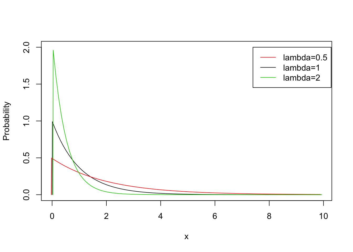
In Figure 5.3.8 the densities of the Exponential distribution are plotted for \(\lambda = 0.5\text{,}\) \(\lambda = 1\text{,}\) and \(\lambda = 2\text{.}\) Notice that with the increase in the value of the parameter then the values of the random variable tends to become smaller. This inverse relation makes sense in connection to the Poisson distribution. Recall that the Poisson distribution corresponds to the total number of occurrences in a unit interval of time when the time between occurrences has an Exponential distribution. A larger expectation \(\lambda\) of the Poisson corresponds to a larger number of occurrences that are likely to take place during the unit interval of time. The larger is the number of occurrences the smaller are the time intervals between occurrences.
Example 5.3.9.
Consider Examples Example 5.2.8 and Example 5.3.5 that deal with rain dropping on a power line. The times between consecutive hits of the line may be modeled by the Exponential distribution. Hence, the time to the first hit has an Exponential distribution. The time between the first and the second hit is also Exponentially distributed, and so on.
Example 5.3.10.
Return to Example 5.2.7 that deals with the radio activity of some element. The total count of decays per second is model by the Poisson distribution. The times between radio active decays is modeled according to the Exponential distribution. The rate \(\lambda\) of that Exponential distribution is equal to the expectation of the total count of decays in one second, i.e. the expectation of the Poisson distribution.

