Introduction to Statistical Thinking

Consider, for example, the probability of obtaining between 1940 and 2060 heads when tossing 4,000 fair coins. Let \(X\) be the total number of heads. The tossing of a coin is a trial with two possible outcomes: “Head” and “Tail”. The probability of a “Head” is 0.5 and there are 4,000 trials. Let us call obtaining a “Head” in a trial a “Success”. Observe that the random variable \(X\) counts the total number of successes. Hence, \(X \sim \mathrm{Binomial}(4000,0.5)\text{.}\)

The probability \(P(1940 \leq X \leq 2060)\) can be computed as the difference between the probability \(P(X \leq 2060)\) of being less or equal to 2060 and the probability \(P(X < 1940)\) of being strictly less than 1940. However, 1939 is the largest integer that is still strictly less than the integer 1940. As a result we get that \(P(X < 1940) = P(X \leq 1939)\text{.}\) Consequently, \(P(1940 \leq X \leq 2060) = P(X \leq 2060) - P(X \leq 1939)\text{.}\)

Applying the function pbinom for the computation of the Binomial cumulative probability, namely the probability of being less or equal to a given value, we get that the probability in the range between 1940 and 2060 is equal to

pbinom(2060,4000,0.5) - pbinom(1939,4000,0.5)

## [1] 0.9442883

This is an exact computation. The Normal approximation produces an approximate evaluation, not an exact computation. The Normal approximation replaces Binomial computations by computations carried out for the Normal distribution. The computation of a probability for a Binomial random variable is replaced by computation of probability for a Normal random variable that has the same expectation and standard deviation as the Binomial random variable.

Notice that if \(X \sim \mathrm{Binomial}(4000,0.5)\) then the expectation is \(\mathbb{E}(X) = 4,000 \times 0.5 = 2,000\) and the variance is \(\mathrm{Var}(X) = 4,000 \times 0.5 \times 0.5 = 1,000\text{,}\) with the standard deviation being the square root of the variance. Repeating the same computation that we conducted for the Binomial random variable, but this time with the function pnorm that is used for the computation of the Normal cumulative probability, we get:

mu <- 4000*0.5
sig <- sqrt(4000*0.5*0.5)
pnorm(2060,mu,sig) - pnorm(1939,mu,sig)

## [1] 0.9442441

Observe that in this example the Normal approximation of the probability (0.9442441) agrees with the Binomial computation of the probability (0.9442883) up to 3 significant digits.

Normal computations may also be applied in order to find approximate percentiles of the Binomial distribution. For example, let us identify the central region that contains for a \(\mathrm{Binomial}(4000,0.5)\) random variable (approximately) 95% of the distribution. Towards that end we can identify the boundaries of the region for the Normal distribution with the same expectation and standard deviation as that of the target Binomial distribution:

qnorm(0.975,mu,sig)
qnorm(0.025,mu,sig)

## [1] 2061.98
## [1] 1938.02

After rounding to the nearest integer we get the interval \([1938,2062]\) as a proposed central region.

In order to validate the proposed region we may repeat the computation under the actual Binomial distribution:

qbinom(0.975,4000,0.5)
qbinom(0.025,4000,0.5)

## [1] 2062
## [1] 1938

Again, we get the interval \([1938,2062]\) as the central region, in agreement with the one proposed by the Normal approximation. Notice that the function qbinom produces the percentiles of the Binomial distribution. It may not come as a surprise to learn that qpois, qunif, qexp compute the percentiles of the Poisson, Uniform and Exponential distributions, respectively.

The ability to approximate one distribution by the other, when computation tools for both distributions are handy, seems to be of questionable importance. Indeed, the significance of the Normal approximation is not so much in its ability to approximate the Binomial distribution as such. Rather, the important point is that the Normal distribution may serve as an approximation to a wide class of distributions, with the Binomial distribution being only one example. Computations that are based on the Normal approximation will be valid for all members in the class of distributions, including cases where we don’t have the computational tools at our disposal or even in cases where we do not know what the exact distribution of the member is! As promised, a more detailed discussion of the Normal approximation in a wider context will be presented in the next chapter.

On the other hand, one need not assume that any distribution is well approximated by the Normal distribution. For example, the distribution of wealth in the population tends to be skewed, with more than 50% of the people possessing less than 50% of the wealth and small percentage of the people possessing the majority of the wealth. The Normal distribution is not a good model for such distribution. The Exponential distribution, or distributions similar to it, may be more appropriate.

In order to complete this section let us look more carefully at the Normal approximations of the Binomial distribution.

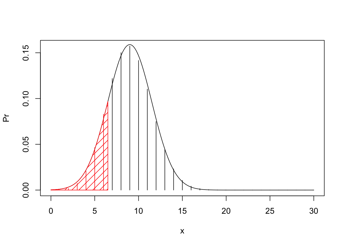
In principle, the Normal approximation is valid when \(n\text{,}\) the number of independent trials in the Binomial distribution, is large. When \(n\) is relatively small the approximation may not be so good. Indeed, take \(X \sim \mathrm{Binomial}(30,0.3)\) and consider the probability \(P(X \leq 6)\text{.}\) Compare the actual probability to the Normal approximation:

pbinom(6,30,0.3)
pnorm(6,30*0.3,sqrt(30*0.3*0.7))

## [1] 0.159523
## [1] 0.1159989

The Normal approximation, which is equal to 0.1159989, is not too close to the actual probability, which is equal to 0.1595230.

A naïve application of the Normal approximation for the \(\mathrm{Binomial}(n,p)\) distribution may not be so good when the number of trials \(n\) is small. Yet, a small modification of the approximation may produce much better results. In order to explain the modification consult Figure 6.3.1 where you will find the bar plot of the Binomial distribution with the density of the approximating Normal distribution superimposed on top of it. The target probability is the sum of heights of the bars that are painted in red. In the naïve application of the Normal approximation we used the area under the normal density which is to the left of the bar associated with the value \(x=6\text{.}\)

Alternatively, you may associate with each bar located at \(x\) the area under the normal density over the interval \([x-0.5, x+0.5]\text{.}\) The resulting correction to the approximation will use the Normal probability of the event \(\{X \leq 6.5\}\text{,}\) which is the area shaded in red. The application of this approximation, which is called continuity correction produces:

pnorm(6.5,30*0.3,sqrt(30*0.3*0.7))

## [1] 0.159523

Observe that the corrected approximation is much closer to the target probability, which is 0.1595230, and is substantially better that the uncorrected approximation which was 0.1159989. Generally, it is recommended to apply the continuity correction to the Normal approximation of a discrete distribution.

Consider the \(\mathrm{Binomial}(n,p)\) distribution. Another situation where the Normal approximation may fail is when \(p\text{,}\) the probability of “Success” in the Binomial distribution, is too close to 0 (or too close to 1). Recall, that for large \(n\) the Poisson distribution emerged as an approximation of the Binomial distribution in such a setting. One may expect that when \(n\) is large and \(p\) is small then the Poisson distribution may produce a better approximation of a Binomial probability. When the Poisson distribution is used for the approximation we call it a Poisson Approximation.

Let us consider an example. Let us analyze 3 Binomial distributions. The expectation in all the distributions is equal to 2 but the number of trials, \(n\text{,}\) vary. In the first case \(n=20\) (and hence \(p=0.1\)), in the second \(n=200\) (and \(p=0.01\)), and in the third \(n=2,000\) (and \(p=0.001\)). In all three cases we will be interested in the probability of obtaining a value less or equal to 3.

The Poisson approximation replaces computations conducted under the Binomial distribution with Poisson computations, with a Poisson distribution that has the same expectation as the Binomial. Since in all three cases the expectation is equal to 2 we get that the same Poisson approximation is used to the three probabilities:

ppois(3,2)

## [1] 0.8571235

The actual Binomial probability in the first case (\(n=20\text{,}\) \(p=0.1\)) and a Normal approximation thereof are:

pbinom(3,20,0.1)
pnorm(3.5,2,sqrt(20*0.1*0.9))

## [1] 0.8670467
## [1] 0.8682238

Observe that the Normal approximation (with a continuity correction) is better than the Poisson approximation in this case.

In the second case (\(n=200\text{,}\) \(p=0.01\)) the actual Binomial probability and the Normal approximation of the probability are:

pbinom(3,200,0.01)
pnorm(3.5,2,sqrt(200*0.01*0.99))

## [1] 0.858034
## [1] 0.856789

Observe that the Poisson approximation that produces 0.8571235 is slightly closer to the target than the Normal approximation. The greater accuracy of the Poisson approximation for the case where \(n\) is large and \(p\) is small is more pronounced in the final case (\(n=2000\text{,}\) \(p=0.001\)) where the target probability and the Normal approximation are:

pbinom(3,2000,0.001)
pnorm(3.5,2,sqrt(2000*0.001*0.999))

## [1] 0.8572138
## [1] 0.8556984

Compare the actual Binomial probability, which is equal to 0.8572138, to the Poisson approximation that produced 0.8571235. The Normal approximation, 0.8556984, is slightly off, but is still acceptable.