Section 7.3 Law of Large Numbers and Central Limit Theorem
The Law of Large Numbers and the Central Limit Theorem are mathematical theorems that describe the sampling distribution of the average for large samples.
Subsection 7.3.1 The Law of Large Numbers
The Law of Large Numbers states that, as the sample size becomes larger, the sampling distribution of the sample average becomes more and more concentrated about the expectation.
Let us demonstrate the Law of Large Numbers in the context of the Uniform distribution. Let the distribution of the measurement \(X\) be \(\mathrm{Uniform}(3,7)\text{.}\) Consider three different sample sizes \(n\text{:}\) \(n=10\text{,}\) \(n=100\text{,}\) and \(n=1000\text{.}\) Let us carry out a simulation similar to the simulations of the previous section. However, this time we run the simulation for the three sample sizes in parallel:
unif.10 <- rep(0,10^5)
unif.100 <- rep(0,10^5)
unif.1000 <- rep(0,10^5)
for(i in 1:10^5) {
  X.samp.10 <- runif(10,3,7)
  unif.10[i] <- mean(X.samp.10)
  X.samp.100 <- runif(100,3,7)
  unif.100[i] <- mean(X.samp.100)
  X.samp.1000 <- runif(1000,3,7)
  unif.1000[i] <- mean(X.samp.1000)
}
Observe that we have produced 3 sequences of length 100,000 each: “
unif.10”, “unif.100”, and “unif.1000”. The first sequence is an approximation of the sampling distribution of an average of 10 independent Uniform measurements, the second approximates the sampling distribution of an average of 100 measurements and the third the distribution of an average of 1000 measurements. The distribution of single measurement in each of the examples is \(\mathrm{Uniform}(3,7)\text{.}\)
Consider the expectation of sample average for the three sample sizes:
mean(unif.10)
mean(unif.100)
mean(unif.1000)
## [1] 5.000141
## [1] 5.000465
## [1] 4.999981
For all sample size the expectation of the sample average is equal to 5, which is the expectation of the \(\mathrm{Uniform}(3,7)\) distribution.
Recall that the variance of the \(\mathrm{Uniform}(a,b)\) distribution is \((b-a)^2/12\text{.}\) Hence, the variance of the given Uniform distribution is \(\Var(X) = (7-3)^2/12 = 16/12 \approx 1.3333\text{.}\) The variances of the sample averages are:
var(unif.10)
var(unif.100)
var(unif.1000)
## [1] 0.1329634
## [1] 0.01341528
## [1] 0.001338488
Notice that the variances decrease with the increase of the sample sizes. The decrease is according to the formula \(\Var(\bar X) = \Var(X)/n\text{.}\)
The variance is a measure of the spread of the distribution about the expectation. The smaller the variance the more concentrated is the distribution around the expectation. Consequently, in agreement with the Law of Large Numbers, the larger the sample size the more concentrated is the sampling distribution of the sample average about the expectation.
Subsection 7.3.2 The Central Limit Theorem (CLT)
The Law of Large Numbers states that the distribution of the sample average tends to be more concentrated as the sample size increases. The Central Limit Theorem (CLT in short) provides an approximation of this distribution.
The deviation between the sample average and the expectation of the measurement tend to decreases with the increase in sample size. In order to obtain a refined assessment of this deviation one needs to magnify it. The appropriate way to obtain the magnification is to consider the standardized sample average, in which the deviation of the sample average from its expectation is divided by the standard deviation of the sample average:
\begin{equation*}
Z = \frac{\bar X - \Expec(\bar X)}{\sqrt{\Var(\bar X)}}\;.
\end{equation*}
Recall that the expectation of the sample average is equal to the expectation of a single random variable (\(\Expec(\bar X) = \Expec(X)\)) and that the variance of the sample average is equal to the variance of a single observation, divided by the sample size (\(\Var(\bar X) = \Var(X)/n\)). Consequently, one may rewrite the standardized sample average in the form:
\begin{equation*}
Z = \frac{\bar X - \Expec(X)}{\sqrt{\Var(X)/n}}= \frac{\sqrt{n}(\bar X - \Expec(X))}{\sqrt{\Var(X)}}\;.
\end{equation*}
The second equality follows from placing in the numerator the square root of \(n\) which divides the term in the denominator. Observe that with the increase of the sample size the decreasing difference between the average and the expectation is magnified by the square root of \(n\text{.}\)
The Central Limit Theorem states that, with the increase in sample size, the sample average converges (after standardization) to the standard Normal distribution.
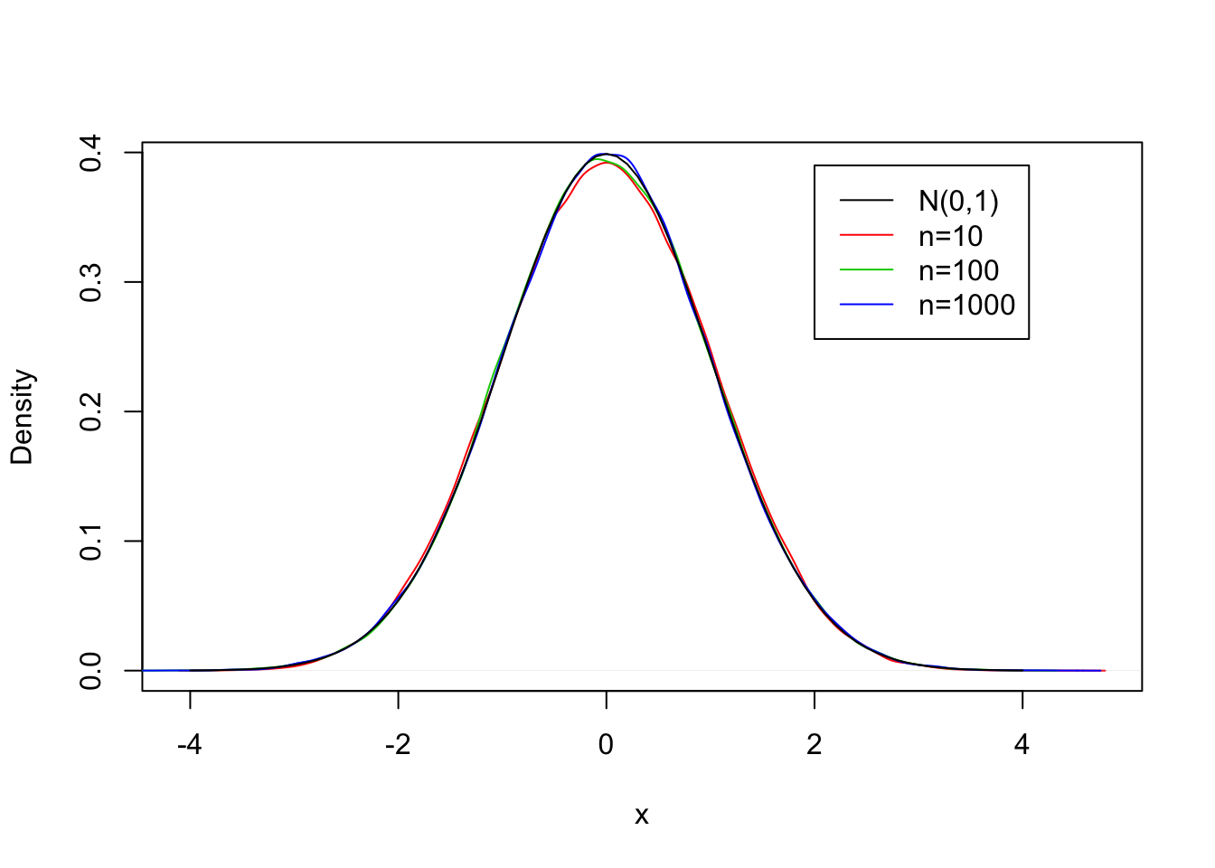
Let us examine the Central Normal Theorem in the context of the example of the Uniform measurement. In Figure 7.3.1 you may find the (approximated) density of the standardized average for the three sample sizes based on the simulation that we carried out previously (as red, green, and blue lines). Along side with these densities you may also find the theoretical density of the standard Normal distribution (as a black line). Observe that the four curves are almost one on top of the other, proposing that the approximation of the distribution of the average by the Normal distribution is good even for a sample size as small as \(n=10\text{.}\)
However, before jumping to the conclusion that the Central Limit Theorem applies to any sample size, let us consider another example. In this example we repeat the same simulation that we did with the Uniform distribution, but this time we take \(\mathrm{Exponential}(0.5)\) measurements instead:
exp.10 <- rep(0,10^5)
exp.100 <- rep(0,10^5)
exp.1000 <- rep(0,10^5)
for(i in 1:10^5) {
  X.samp.10 <- rexp(10,0.5)
  exp.10[i] <- mean(X.samp.10)
  X.samp.100 <- rexp(100,0.5)
  exp.100[i] <- mean(X.samp.100)
  X.samp.1000 <- rexp(1000,0.5)
  exp.1000[i] <- mean(X.samp.1000)
}
The expectation of an \(\mathrm{Exponential}(0.5)\) random variable is \(\Expec(X) = 1/\lambda = 1/0.5 = 2\) and the variance is \(\Var(X) = 1/\lambda^2 = 1/(0.5)^2 = 4\text{.}\) Observe below that the expectations of the sample averages are equal to the expectation of the measurement and the variances of the sample averages follow the relation \(\Var(\bar X) = \Var (X)/n\text{:}\)
mean(exp.10)
mean(exp.100)
mean(exp.1000)
## [1] 1.999011
## [1] 2.000074
## [1] 2.000183
So the expectations of the sample average are all equal to 2. For the variance we get:
var(exp.10)
var(exp.100)
var(exp.1000)
## [1] 0.3980615
## [1] 0.04012221
## [1] 0.004005182
Which is in agreement with the decrease proposed by the theory,
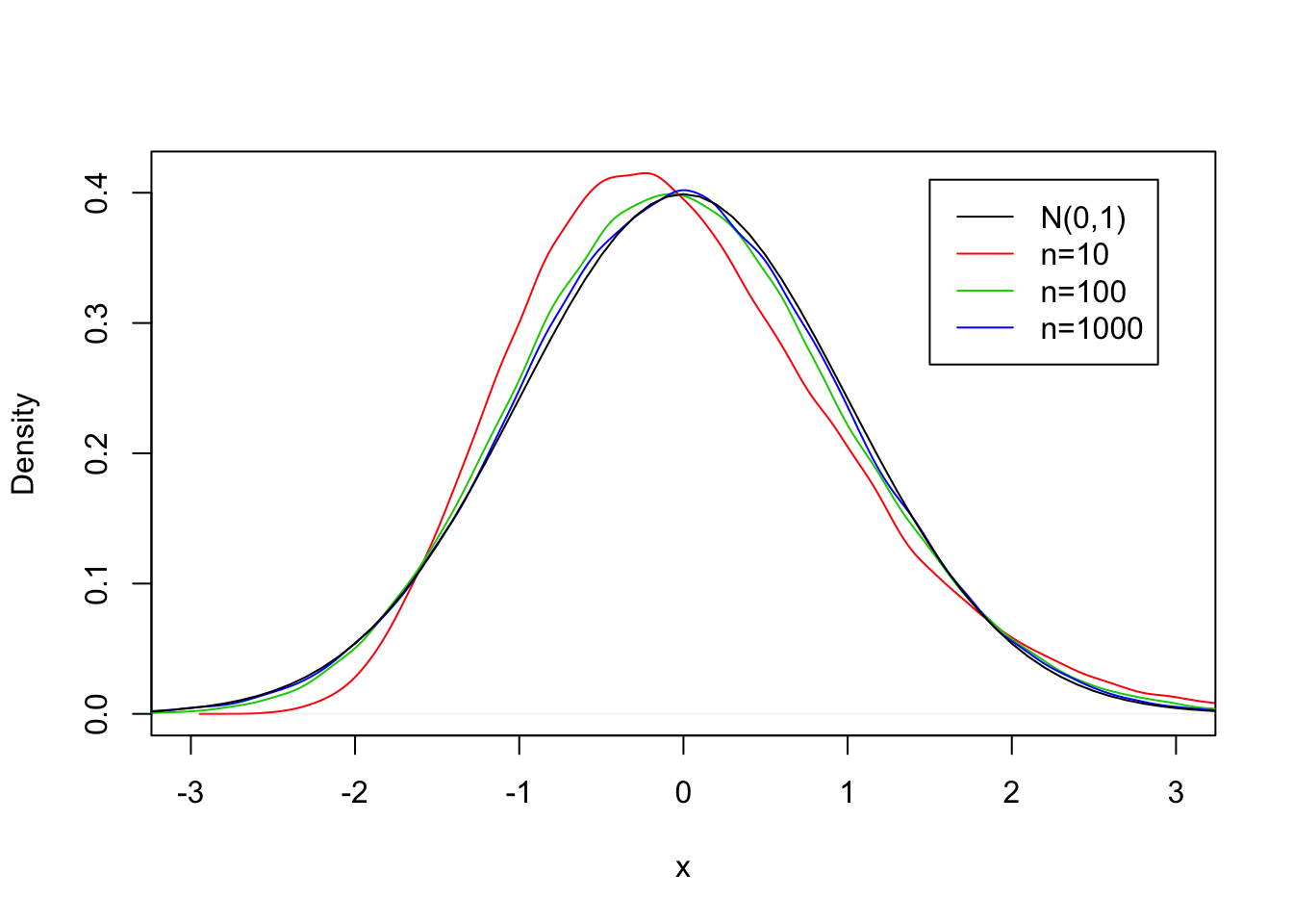
However, when one examines the densities of the sample averages in Figure 7.3.2 one may see a clear distinction between the sampling distribution of the average for a sample of size 10 and the normal distribution (compare the red curve to the black curve. The match between the green curve that corresponds to a sample of size \(n=100\) and the black line is better, but not perfect. When the sample size is as large as \(n=1000\) (the blue curve) then the agreement with the normal curve is very good.
Subsection 7.3.3 Applying the Central Limit Theorem
The conclusion of the Central Limit Theorem is that the sampling distribution of the sample average can be approximated by the Normal distribution, regardless what is the distribution of the original measurement, but provided that the sample size is large enough. This statement is very important, since it allows us, in the context of the sample average, to carry out probabilistic computations using the Normal distribution even if we do not know the actual distribution of the measurement. All we need to know for the computation are the expectation of the measurement, its variance (or standard deviation) and the sample size.
The theorem can be applied whenever probability computations associated with the sampling distribution of the average are required. The computation of the approximation is carried out by using the Normal distribution with the same expectation and the same standard deviation as the sample average.
An example of such computation was conducted in Subsection 7.2.3 where the central interval that contains 95% of the sampling distribution of a Binomial average was required. The 2.5%- and the 97.5%-percentiles of the Normal distribution with the same expectation and variance as the sample average produced boundaries for the interval. These boundaries were in good agreement with the boundaries produced by the simulation. More examples will be provided in the Solved Exercises of this chapter and the next one.
With all its usefulness, one should treat the Central Limit Theorem with a grain of salt. The approximation may be valid for large samples, but may be bad for samples that are not large enough. When the sample is small a careless application of the Central Limit Theorem may produce misleading conclusions.

