Introduction to Statistical Thinking

Before the file is read into R you should obtain a copy of the file and store it in some directory on the computer and read the file from that directory. We recommend that you create a special directory in which you keep all the material associated with this course. In the explanations provided below we assume that the directory to which the file is stored in called “IntroStat”.

Files in the CSV format are ordinary text files. They can be created manually or as a result of converting data stored in a different format into this particular format. A common way to produce, browse and edit CSV files is by the use of a standard electronic spreadsheet programs such as Excel or Calc. The Excel spreadsheet is part of the Microsoft’s Office suite. The Calc spreadsheet is part of the free LibreOffice suite. Note however that you should never edit raw data files directly. Keep them in a separate directory and never overwrite them with changes. Any changes you make to the data should be retraceable and documented through R-scripts and the changed data should be saved under a different name.

Opening a CSV file by a spreadsheet program displays a spreadsheet with the content of the file. Values in the cells of the spreadsheet may be modified directly. (However, when saving, one should pay attention to save the file in the CVS format.) Similarly, new CSV files may be created by the entering of the data in an empty spreadsheet. The first row should include the name of the variable, preferably as a single character string with no empty spaces. The following rows may contain the data values associated with this variable. When saving, the spreadsheet should be saved in the CSV format by the use of the “” dialog and choosing there the option of CSV in the “Save by Type” selection.

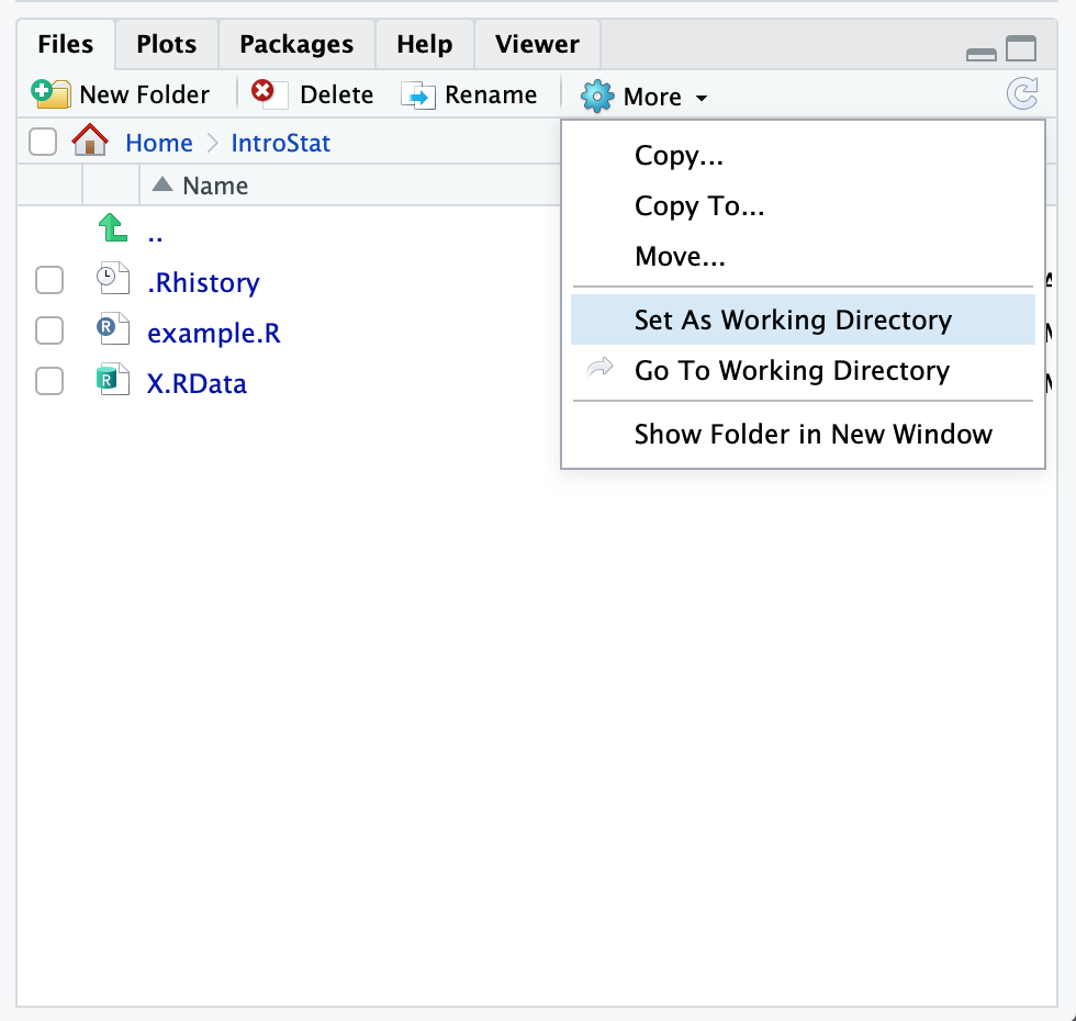
After saving a file with the data in a directory, R should be notified where the file is located in order to be able to read it. A simple way of doing so is by setting the directory with the file as R’s working directory. The working directory is the first place R is searching for files. Files produced by R are saved in that directory. In RStudio one may set the working directory of the active R session to be some target directory in the “Files” panel The dialog is opened by clicking on “More” on the left hand side of the toolbar on the top of the Files panel. In the menu that opens selecting the option of “Set As Working Directory” will start the dialog. (See Figure 2.3.1.) Browsing via this dialog window to the directory of choice, selecting it, and approving the selection by clicking the “OK” bottom in the dialog window will set the directory of choice as the working directory of R.

A full statistical ananlysis will typically involve a non-negligible number of steps. Retracing these steps in retrospect is often difficult without proper documentation. So while working from the R-console is a good way to develop (steps) in an analysis, you will need a way to document your work in order for your the analysis to be reproducible. Rather than to work only from the R-console (and change the working directory every time that R is opened manually), it is better to organize your R-code in so-called scripts. R-scripts are plain text files which contain the R-commands that perform your analysis. Executing these scripts will perform your full analysis and thereby make your work reproducible.

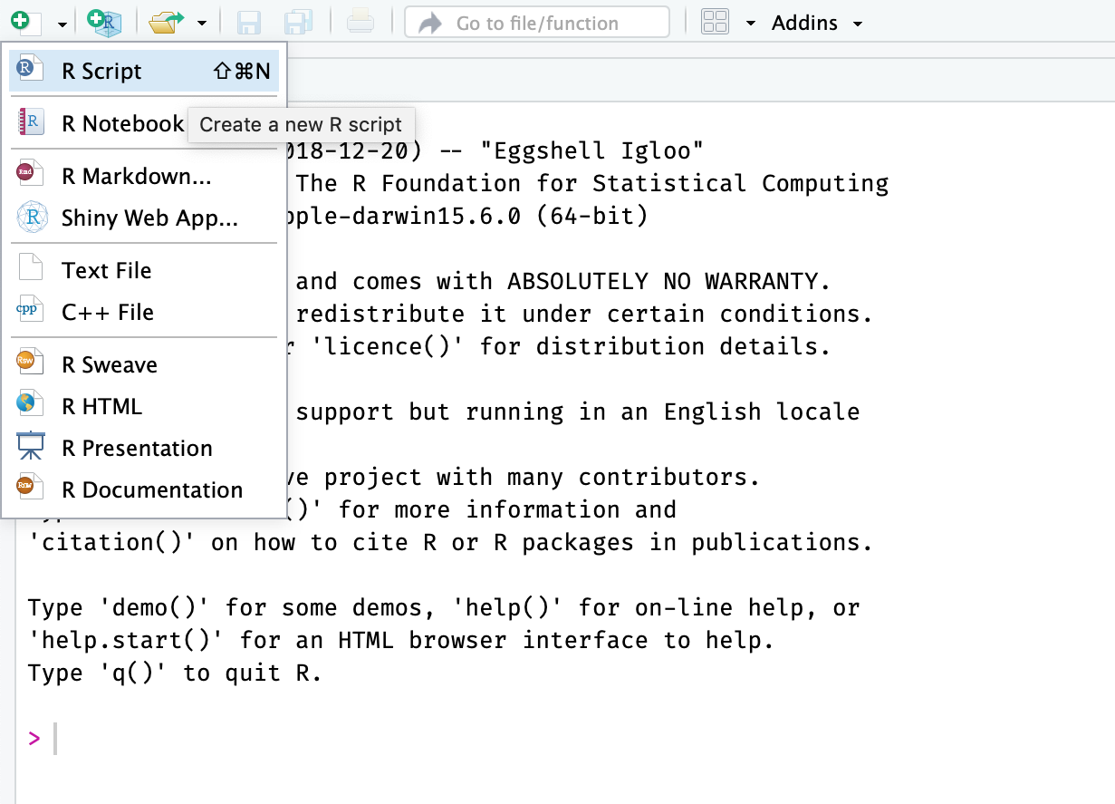
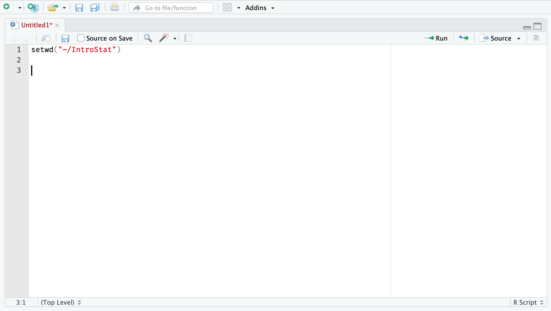
Figure 2.3.2 shows how to create an R-script in RStudio. This is done by clicking on the first button on the main toolbar in RStudio. This will popup a menu where you can click on R-script. RStudio will then create a new empty R-script in the editing panel as shown in Figure 2.3.3. Here you can add the R-commands that will perform your analysis. Make sure to save your new script. Finally note that you can select one or several lines in your R-script and click on the Run’ button in the toolbar to execute them in the R-console.

In the rest of this book we assume that a designated directory is set as R’s working directory and that all external files that need to be read into R, such as “ex1.csv” for example, are saved in that working directory. Once a working directory has been set then the history of subsequent R sessions is stored in that directory. Hence, if you choose to save the image of the session when you end the session then objects created in the session will be uploaded the next time the R Console is opened.

Now that a copy of the file “ex1.csv” is placed in the working directory we would like to read its content into R. Reading of files in the CSV format can be carried out with the R function “read.csv”. To read the file of the example we run the following line of code in the R Console panel:

ex.1 <- read.csv("_data/ex1.csv")

The function “read.csv” takes as an input argument the address of a CSV file and produces as output a data frame object with the content of the file. Notice that the address is placed between double-quotes. If the file is located in the working directory then giving the name of the file as an address is sufficient

¹

If the file is located in a different directory than the complete address, including the path to the file, should be provided. The file need not reside on the computer. One may provide, for example, a URL (an internet address) as the address. Thus, instead of saving the file of the example on the computer one may read its content into an R object by using the line of code “ex.1 <- read.csv(http://pluto.huji.ac.il/~msby/StatThink/Datasets/ex1.csv)” instead of the code that we provide and the working method that we recommend to follow.

.

Consider the content of that R object “ex.1” that was created by the previous expression, by inspecting the first part using the function “head()”:

head(ex.1)

##        id    sex height
## 1 5696379 FEMALE    182
## 2 3019088   MALE    168
## 3 2038883   MALE    172
## 4 1920587 FEMALE    154
## 5 6006813   MALE    174
## 6 4055945 FEMALE    176

The object “ex.1”, the output of the function “read.csv” is a data frame. Data frames are the standard tabular format of storing statistical data. The columns of the table are called variables and correspond to measurements. In this example the three variables are:

When the values of the variable are numerical we say that it is a quantitative variable or a numeric variable. On the other hand, if the variable has qualitative or level values we say that it is a factor. In the given example, sex is a factor and height is a numeric variable.

The rows of the table are called observations and correspond to the subjects. In this data set there are 100 subjects, with subject number 1, for example, being a female of height 182 cm and identifying number 5696379. Subject number 98, on the other hand, is a male of height 195 cm and identifying number 9383288.

The columns of R data frames represent variables, i.e. measurements recorded for each of the subjects in the sample. R associates with each variable a type that characterizes the content of the variable. The two major types are

Factors are the result of categorizing or describing attributes of a population. Hair color, blood type, ethnic group, the car a person drives, and the street a person lives on are examples of qualitative data. Qualitative data are generally described by words or letters. For instance, hair color might be black, dark brown, light brown, blonde, gray, or red. Blood type might be AB+, O-, or B+. Qualitative data are not as widely used as quantitative data because many numerical techniques do not apply to the qualitative data. For example, it does not make sense to find an average hair color or blood type.

Quantitative data are always numbers and are usually the data of choice because there are many methods available for analyzing such data. Quantitative data are the result of counting or measuring attributes of a population. Amount of money, pulse rate, weight, number of people living in your town, and the number of students who take statistics are examples of quantitative data.

Quantitative data may be either discrete or continuous. All data that are the result of counting are called quantitative discrete data. These data take on only certain numerical values. If you count the number of phone calls you receive for each day of the week, you may get results such as 0, 1, 2, 3, etc. On the other hand, data that are the result of measuring on a continuous scale are quantitative continuous data, assuming that we can measure accurately. Measuring angles in radians may result in the numbers \(\frac{\pi}{6}\text{,}\) \(\frac{\pi}{3}\text{,}\) \(\frac{\pi}{2}\text{,}\) \(\pi\text{,}\) \(\frac{3\pi}{4}\text{,}\) etc. If you and your friends carry backpacks with books in them to school, the numbers of books in the backpacks are discrete data and the weights of the backpacks are continuous data.

The data are the number of books students carry in their backpacks. You sample five students. Two students carry 3 books, one student carries 4 books, one student carries 2 books, and one student carries 1 book. The numbers of books (3, 4, 2, and 1) are the quantitative discrete data.

The data are the weights of the backpacks with the books in it. You sample the same five students. The weights (in pounds) of their backpacks are 6.2, 7, 6.8, 9.1, 4.3. Notice that backpacks carrying three books can have different weights. Weights are quantitative continuous data because weights are measured.

The data are the colors of backpacks. Again, you sample the same five students. One student has a red backpack, two students have black backpacks, one student has a green backpack, and one student has a gray backpack. The colors red, black, black, green, and gray are qualitative data.

The distinction between continuous and discrete numeric data is not reflected usually in the statistical method that are used in order to analyze the data. Indeed, R does not distinguish between these two types of numeric data and store them both as “numeric”. Consequently, we will also not worry about the specific categorization of numeric data and treat them as one. On the other hand, emphasis will be given to the difference between numeric and factors data.

One may collect data as numbers and report it categorically. For example, the quiz scores for each student are recorded throughout the term. At the end of the term, the quiz scores are reported as A, B, C, D, or F. On the other hand, one may code categories of qualitative data with numerical values and report the values. The resulting data should nonetheless be treated as a factor.

As default, R saves variables that contain non-numeric values as factors. Otherwise, the variables are saved as numeric. The variable type is important because different statistical methods are applied to different data types. Hence, one should make sure that the variables that are analyzed have the appropriate type. Especially that factors using numbers to denote the levels are labeled as factors. Otherwise R will treat them as quantitative data.