Section 1.6 The R Programming Environment
The
R Programming Environment is a widely used open source system for statistical analysis and statistical programming. It includes thousands of functions for the implementation of both standard and exotic statistical methods and it is probably the most popular system in the academic world for the development of new statistical tools. We will use R in order to apply the statistical methods that will be discussed in the book to some example data sets and in order to demonstrate, via simulations, concepts associated with probability and its application in statistics.
The demonstrations in the book involve very basic
R programming skills and the applications are implemented using, in most cases, simple and natural code. A detailed explanation will accompany the code that is used.
Learning
R, like the learning of any other programming language, can be achieved only through practice. Hence, we strongly recommend that you not only read the code presented in the book but also run it yourself, in parallel to the reading of the provided explanations. Moreover, you are encouraged to play with the code: introduce changes in the code and in the data and see how the output changes as a result. One should not be afraid to experiment. At worst, the computer may crash or freeze. In both cases, restarting the computer will solve the problem …
You may download
R from the R project home page www.r-project.org and install it on the computer that you are using.
In addition to installing
R we recommend that you also install RStudio www.rstudio.com. RStudio is an integrated development environment (IDE) for R. It includes a console, syntax-highlighting editor that supports direct code execution, as well as tools for plotting, history, debugging and workspace management.
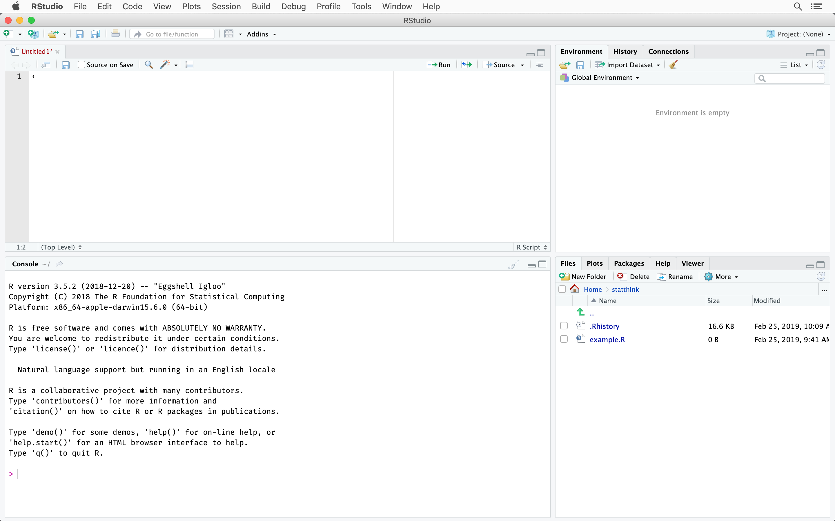
The screenshot in Figure 1.6.1 shows the RStudio interface. There are four panels. The top-left panel is the editor, the bottom-left panel shows the
R-Console. The two right panels show the R-environment, history, file browser, plot panel and help viewer among others.
Subsection 1.6.1 Some Basic R Commands
R is an object-oriented programming system. During the session you may create and manipulate objects by the use of functions that are part of the basic installation. You may also use the R programming language. Most of the functions that are part of the system are themselves written in the R language and one may easily write new functions or modify existing functions to suit specific needs.
Let us start by opening
RStudio. It is good practice to have a separate folder for each project where you will store your data and R-code. We have a folder called IntroStat. When starting a R or RStudio-session it is good practice to set the current working directory to your project directory using the “setwd” function for example like this:
setwd("~/IntroStat")
Now we are ready to run our first
R-command. Type in the R-Console panel, immediately after the “>” prompt, the expression “1+2” and then hit the Return key. (Do not include the double quotation in the expression that you type!):
1 + 2
The prompt “
>” indicates that the system is ready to receive commands. Writing an expression, such as “1+2”, and hitting the Return key sends the expression to be executed. The execution of the expression may produce an object, in this case an object that is composed of a single number, the number “3”.
Whenever required, the
R system takes an action. If no other specifications are given regarding the required action then the system will apply the pre-programmed action. This action is called the default action. In the case of hitting the Return key after the expression that we wrote the default is to display the produced object on the screen.
Next, let us demonstrate . For that we will use the function “
R in a more meaningful way by using it in order to produce the bar-plot of Figure 1.3.1. First we have to input the data. We will produce a sequence of numbers that form the data1
In
R, a sequence of numbers is called a vector. However, we will use the term sequence to refer to vectors.
c” that combines its arguments and produces a sequence with the arguments as the components of the sequence. Write the expression:
c(5,5.5,6,6,6,6.5,6.5,6.5,6.5,7,7,8,8,9)
at the prompt and hit return.
The function “
c” is an example of an R function. A function has a name, “c” in this case, that is followed by brackets that include the input to the function. We call the components of the input the arguments of the function. Arguments are separated by commas. A function produces an output, which is typically an R object. In the current example an object of the form of a sequence was created and, according to the default application of the system, was sent to the screen and not saved.
If we want to create an object for further manipulation then we should save it and give it a name. For example, if we want to save the vector of data under the name “
X” we may write the following expression at the prompt (and then hit return):
X <- c(5,5.5,6,6,6,6.5,6.5,6.5,6.5,7,7,8,8,9)
The arrow that appears after the “
X” is produced by typing the less than key “<” followed by the minus key “-”. This arrow is the assignment operator.
Observe that you may save typing by calling and editing lines of code that were processes in an earlier part of the session. One may browse through the lines using the up and down arrows on the right-hand side of the keyboard and use the right and left arrows to move along the line presented at the prompt. For example, the last expression may be produced by finding first the line that used the function “
c” with the up and down arrow and then moving to the beginning of the line with the left arrow. At the beginning of the line all one has to do is type “X <- ” and hit the Return key.
Notice that no output was sent to the screen. Instead, the output from the “
c” function was assigned to an object that has the name “X”. A new object by the given name was formed and it is now available for further analysis. In order to verify this you may write “X” at the prompt and hit return:
X
The content of the object “
X” is sent to the screen, which is the default output. Notice that we have not changed the given object, which is still in the memory.
The object “
X” is in the memory, but it is not saved on the hard disk. With the end of the session the objects created in the session are erased unless specifically saved.
You can save objects with the “
save” function
save(X, file = "X.RData")
To see whether this worked, delete the object
X from your environment using the function “rm”, load your saved object using the “load” function, and print its contents to check whether we successfully restored it:
rm(X)
load("X.RData")
X
We used a capital letter to name the object. We could have used a small letter just as well or practically any combination of letters. However, you should note that
R distinguishes between capital and small letter. Hence, typing “x” in the console window and hitting return will produce an error message:
x
An object named “
x” does not exist in the R system and we have not created such object. The object “X”, on the other hand, does exist.
Names of functions that are part of the system are fixed but you are free to choose a name to objects that you create. For example, if one wants to create an object by the name “
my.vector” that contains the numbers 3, 7, 3, 3, and -5 then one may write the expression “my.vector <- c(3,7,3,3,-5)” at the prompt and hit the Return key.
If we want to produce a table that contains a count of the frequency of the different values in our data we can apply the function “
table” to the object “X” (which is the object that contains our data):
table(X)
Notice that the output of the function “
table” is a table of the different levels of the input vector and the frequency of each level. This output is yet another type of an object.
The bar-plot of Figure 1.3.1 can be produced by the application of the function “
plot” to the object that is produced as an output of the function “table”:
plot(table(X))
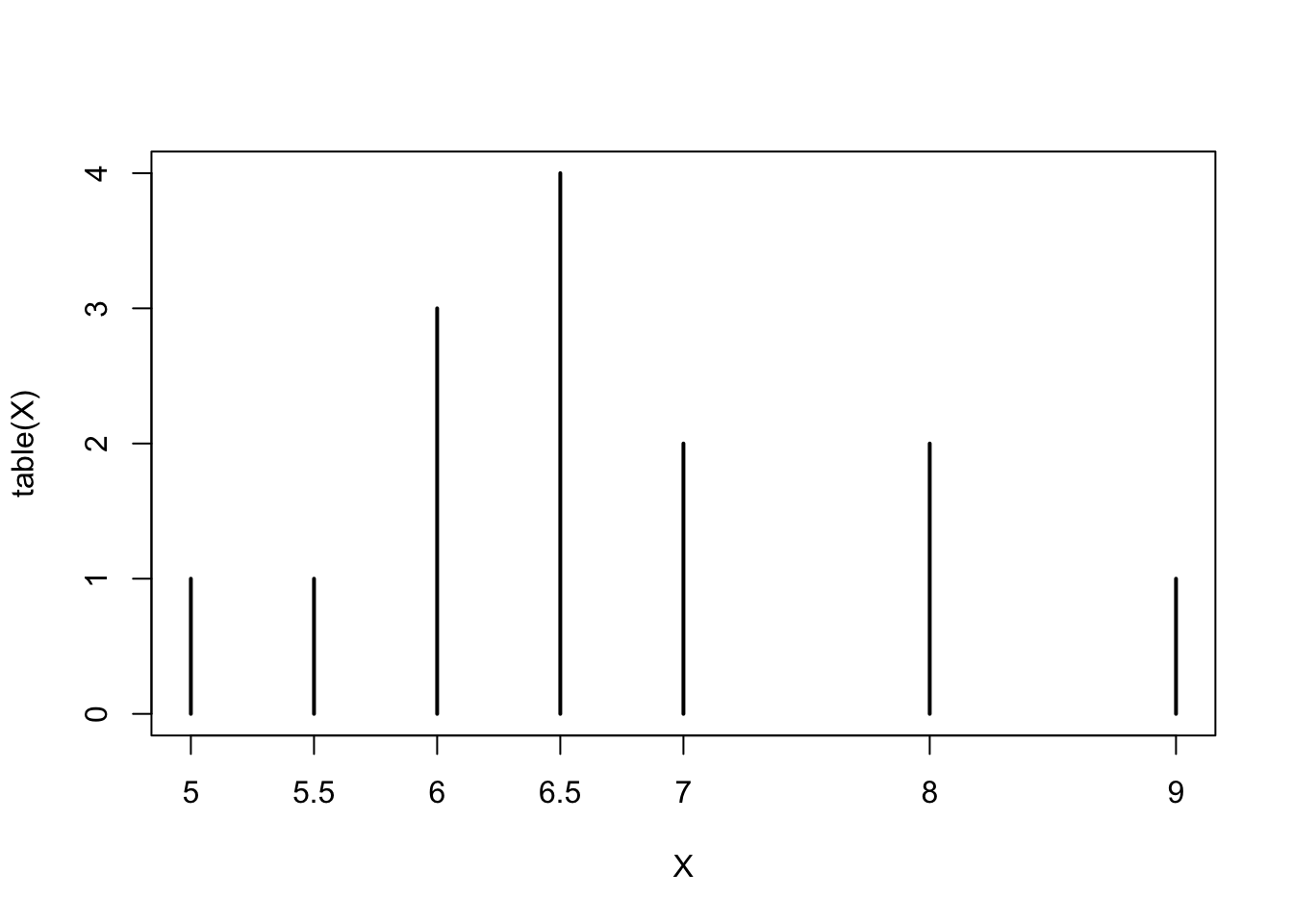
This plot is practically identical to the plot in Figure 1.3.1. The only difference is in the names given to the axes. These names were changed in Figure 1.3.1 for clarity.
Clearly, if one wants to produce a bar-plot to other numerical data all one has to do is replace in the expression
plot(table(X)) the object X by an object that contains the other data. For example, to plot the data in my.vector you may use plot(table(my.vector)).

