Exercises

Section 14.5 Exercises

Checkpoint 14.5.1.

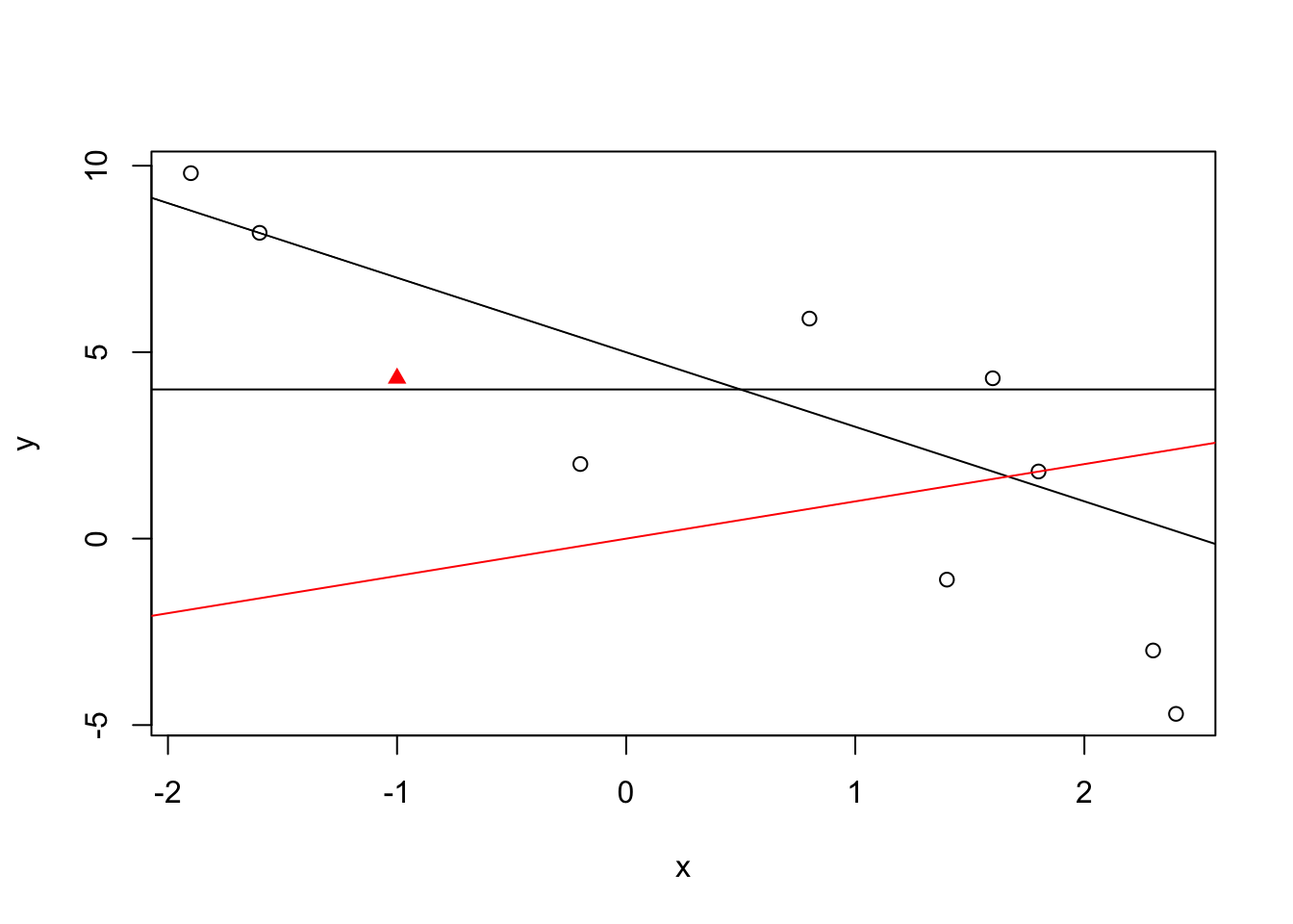
Figure 14.5.3 presents 10 points and three lines. One of the lines is colored red and one of the points is marked as a red triangle. The points in the plot refer to the data frame in Table 14.5.2 and the three lines refer to the linear equations:

1. $y = 4$

2. $y = 5 - 2x$

3. $y = x$

You are asked to match the marked line to the appropriate linear equation and match the marked point to the appropriate observation:

🔗

1. Which of the three equations, 1, 2 or 3, describes the line marked in red?

🔗

2. The point marked with a red triangle represents which of the observations. (Identify the observation number.)

🔗

Table 14.5.2. Points

🔗

Observation	$x$	$y$
1	2.3	-3.0
2	-1.9	9.8
3	1.6	4.3
4	-1.6	8.2
5	0.8	5.9
6	-1.0	4.3
7	-0.2	2.0
8	2.4	-4.7
9	1.8	1.8
10	1.4	-1.1

🔗

Scatter plot with 10 points and three lines, one marked in red — Figure 14.5.3. Lines and Points
🔗

Checkpoint 14.5.4.

Assume a regression model that describes the relation between the expectation of the response and the value of the explanatory variable in the form:

🔗

\begin{equation*} \Expec(Y_i) = 2.13 \cdot x_i - 3.60\;. \end{equation*}

1. What is the value of the intercept and what is the value of the slope in the linear equation that describes the model?

🔗

2. Assume the $x_1 = 5.5\text{,}$ $x_2 = 12.13\text{,}$ $x_3 = 4.2\text{,}$ and $x_4 = 6.7\text{.}$ What is the expected value of the response of the 3rd observation?

🔗

Checkpoint 14.5.5.

The file “aids.csv” contains data on the number of diagnosed cases of Aids and the number of deaths associated with Aids among adults and adolescents in the United States between 1981 and 2002

The data is taken from Table 1 in section “Practice in Linear Regression” of the online Textbook “Collaborative Statistics” (Connexions. March 22, 2010. http://cnx.org/content/col10522/1.38/) by Barbara Illowsky and Susan Dean.

. The file can be found on the internet at http://pluto.huji.ac.il/~msby/StatThink/Datasets/aids.csv.

🔗

The file contains 3 variables: The variable “year” that tells the relevant year, the variable “diagnosed” that reports the number of Aids cases that were diagnosed in each year, and the variable “deaths” that reports the number of Aids related deaths in each year. The following questions refer to the data in the file:

🔗

1. Consider the variable “deaths” as response and the variable “diagnosed” as an explanatory variable. What is the slope of the regression line? Produce a point estimate and a confidence interval. Is it statistically significant (namely, significantly different than 0)?

🔗

2. Plot the scatter plot that is produced by these two variables and add the regression line to the plot. Does the regression line provided a good description of the trend in the data?

🔗

3. Consider the variable “diagnosed” as the response and the variable “year” as the explanatory variable. What is the slope of the regression line? Produce a point estimate and a confidence interval. Is the slope in this case statistically significant?

🔗

4. Plot the scatter plot that is produced by the later pair of variables and add the regression line to the plot. Does the regression line provided a good description of the trend in the data?

🔗

Checkpoint 14.5.6.

Below are the percents of the U.S. labor force (excluding self-employed and unemployed) that are members of a labor union

Taken from Homework section in the chapter on linear regression of the online Textbook “Collaborative Statistics” (Connexions. March 22, 2010. http://cnx.org/content/col10522/1.38/) by Barbara Illowsky and Susan Dean.

. We use this data in order to practice the computation of the regression coefficients.

🔗

Table 14.5.7. Percent of Union Members

🔗

year	percent
1945	35.5
1950	31.5
1960	31.4
1970	27.3
1980	21.9
1986	17.5
1993	15.8

1. Produce the scatter plot of the data and add the regression line. Is the regression model reasonable for this data?

🔗

2. Compute the sample averages and the sample standard deviations of both variables. Compute the covariance between the two variables.

🔗

3. Using the summaries you have just computed, recompute the coefficients of the regression model.

🔗

Checkpoint 14.5.8.

Assume a regression model was fit to some data that describes the relation between the explanatory variable $x$ and the response $y\text{.}$ Assume that the coefficients of the fitted model are $a=2.5$ and $b=-1.13\text{,}$ for the intercept and the slope, respectively. The first 4 observations in the data are $(x_1,y_1) = (5.5,3.22)\text{,}$ $(x_2,y_2) = (12.13,-6.02)\text{,}$ $(x_3,y_3) = (4.2,-8.3)\text{,}$ and $(x_4,y_4) = (6.7,0.17)\text{.}$

🔗

1. What is the estimated expectation of the response for the 4th observation?

🔗

2. What is the residual from the regression line for the 4th observation?

🔗

Checkpoint 14.5.9.

In Chapter 13 we analyzed an example that involved the difference between fuel consumption in highway and city driving conditions as the response

The response was computed using the expression “cars$highway.mpg - cars$city.mpg”

. The explanatory variable was a factor that was produced by splitting the cars into two weight groups. In this exercise we would like to revisit this example. Here we use the weight of the car directly as an explanatory variable. We also consider the size of the engine as an alternative explanatory variable and compare between the two regression models.

🔗

1. Fit the regression model that uses the variable “curb.weight” as an explanatory variable. Is the slope significantly different than 0? What fraction of the standard deviation of the response is explained by a regression model involving this variable?

🔗

2. Fit the regression model that uses the variable “engine.size” as an explanatory variable. Is the slope significantly different than 0? What fraction of the standard deviation of the response is explained by a regression model involving this variable?

🔗

3. Which of the two models fits the data better?

🔗

Prev Top Next