Section 3.3 Measures of the Center of Data
The two most widely used measures of the central location of the data are the mean (average) and the median. To calculate the average weight of 50 people one should add together the 50 weights and divide the result by 50. To find the median weight of the same 50 people, one may order the data and locate a number that splits the data into two equal parts. The median is generally a better measure of the center when there are extreme values or outliers because it is not affected by the precise numerical values of the outliers. Nonetheless, the mean is the most commonly used measure of the center.
We shall use small Latin letters such as \(x\) to mark the sequence of data. In such a case we may mark the sample mean by placing a bar over the \(x\text{:}\) \(\bar x\) (pronounced “\(x\) bar”).
The mean can be calculated by averaging the data points or it also can be calculated with the relative frequencies of the values that are present in the data. In the latter case one multiplies each distinct value by its relative frequency and then sum the products across all values. To see that both ways of calculating the mean are the same, consider the data:
\begin{equation*}
1,\; 1,\; 1,\; 2,\; 2,\; 3,\; 4,\; 4,\; 4,\; 4,\; 4
\end{equation*}
In the first way of calculating the mean we get:
\begin{equation*}
\bar x = \frac{1 + 1 + 1 + 2 + 2 + 3 + 4 + 4 + 4 + 4 + 4}{11} = 2.7\;.
\end{equation*}
Alternatively, we may note that the distinct values in the sample are 1, 2, 3, and 4 with relative frequencies of 3/11, 2/11, 1/11 and 5/11, respectively. The alternative method of computation produces:
\begin{equation*}
\bar x = 1\times \frac{3}{11} + 2 \times \frac{2}{11} + 3 \times \frac{1}{11} + 4 \times \frac{5}{11} = 2.7\;.
\end{equation*}
Subsection 3.3.1 Skewness, the Mean and the Median
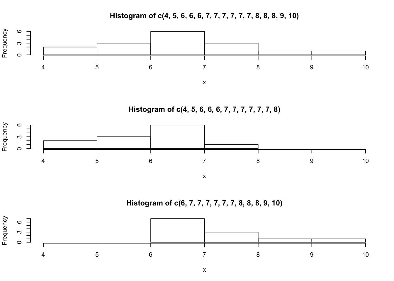
Consider the following data set:
\begin{equation*}
4,\; 5,\; 6,\; 6,\; 6,\; 7,\; 7,\; 7,\; 7,\; 7,\; 7,\; 8,\; 8,\; 8,\; 9,\; 10
\end{equation*}
This data produces the upper most histogram in Figure 3.3.1. Each interval has width one and each value is located at the middle of an interval. The histogram displays a symmetrical distribution of data. A distribution is symmetrical if a vertical line can be drawn at some point in the histogram such that the shape to the left and to the right of the vertical line are mirror images of each other.
Let us compute the mean and the median of this data:
x <- c(4,5,6,6,6,7,7,7,7,7,7,8,8,8,9,10)
mean(x)
median(x)
## [1] 7
## [1] 7
The mean and the median are each 7 for these data. In a perfectly symmetrical distribution, the mean and the median are the same.
1
In the case of a symmetric distribution the vertical line of symmetry is located at the mean, which is also equal to the median.
The functions “
mean” and “median” were used in order to compute the mean and median. Both functions expect a numeric sequence as an input and produce the appropriate measure of centrality of the sequence as an output.
The histogram for the data:
\begin{equation*}
4,\; 5,\; 6,\; 6,\; 6,\; 7,\; 7,\; 7,\; 7,\; 7,\; 7,\; 8
\end{equation*}
is not symmetrical and is displayed in the middle of Figure 3.3.1. The right-hand side seems “chopped off” compared to the left side. The shape of the distribution is called skewed to the left because it is pulled out towards the left.
Let us compute the mean and the median for this data:
x <- c(4,5,6,6,6,7,7,7,7,7,7,8)
mean(x)
median(x)
## [1] 6.416667
## [1] 7
(Notice that the original data is replaced by the new data when object
x is reassigned.) The median is still 7, but the mean is less than 7. The relation between the mean and the median reflects the skewing.
Consider yet another set of data:
\begin{equation*}
6,\; 7,\; 7,\; 7,\; 7,\; 7,\; 7,\; 8,\; 8,\; 8,\; 9,\; 10
\end{equation*}
The histogram for the data is also not symmetrical and is displayed at the bottom of Figure 3.3.1. Notice that it is skewed to the right. Compute the mean and the median:
x <- c(6,7,7,7,7,7,7,8,8,8,9,10)
mean(x)
median(x)
## [1] 7.583333
## [1] 7
The median is yet again equal to 7, but this time the mean is greater than 7. Again, the mean reflects the skewing.
In summary, if the distribution of data is skewed to the left then the mean is less than the median. If the distribution of data is skewed to the right then the median is less than the mean.
Examine the data on the height in “
ex.1”:
mean(ex.1$height)
median(ex.1$height)
## [1] 170.11
## [1] 171
Observe that the histogram of the height (Figure 3.2.1) is skewed to the left. This is consistent with the fact that the mean is less than the median.

