Integrated Applications

Section 8.3 Integrated Applications

The main message of the Central Limit Theorem is that for the sample average we may compute probabilities based on the Normal distribution and obtain reasonable approximations, provided that the sample size is not too small. All we need to figure out for the computations are the expectation and variance of the underlying measurement. Otherwise, the exact distribution of that measurement is irrelevant. Let us demonstrate the applicability of the Central Limit Theorem in two examples.

🔗

Example 8.3.1. Stress Study with Continuous Distribution.

A study involving stress is done on a college campus among the students. The stress scores follow a (continuous) Uniform distribution with the lowest stress score equal to 1 and the highest equal to 5. Using a sample of 75 students, find:

🔗

The probability that the average stress score for the 75 students is less than 2.
🔗

🔗
The 90th percentile for the average stress score for the 75 students.
🔗

🔗
The probability that the total of the 75 stress scores is less than 200.
🔗

🔗
The 90th percentile for the total stress score for the 75 students.
🔗

🔗

Solution.

Denote by $X$ the stress score of a random student. We are given that $X \sim \text{Uniform}(1,5)\text{.}$ We use the formulas $\mathbb{E}(X) = (a+b)/2$ and $\text{Var}(X) = (b-a)^2/12$ in order to obtain the expectation and variance of a single observation and then we use the relations $\mathbb{E}(\bar X) = \mathbb{E}(X)$ and $\text{Var}(\bar X) = \text{Var}(X)/n$ to translate these results to the expectation and variance of the sample average:

🔗

a <- 1
b <- 5
n <- 75
mu.bar <- (a+b)/2
sig.bar <- sqrt((b-a)^2/(12*n))
mu.bar
sig.bar

## [1] 3
## [1] 0.1333333

After obtaining the expectation and the variance of the sample average we can forget about the Uniform distribution and proceed only with the R functions that are related to the Normal distribution. By the Central Limit Theorem we get that the distribution of the sample average is approximately $\text{Normal}(\mu, \sigma^2)\text{,}$ with $\mu$ = mu.bar and $\sigma$ = sig.bar.

🔗

In the Question 1.1 we are asked to find the value of the cumulative distribution function of the sample average at $x=2\text{:}$

🔗

pnorm(2,mu.bar,sig.bar)

## [1] 7.655734e-15

The goal of Question 1.2 is to identify the 90%-percentile of the sample average:

🔗

qnorm(0.9,mu.bar,sig.bar)

## [1] 3.170874

The sample average is equal to the total sum divided by the number of observations, $n=75$ in this example. The total sum is less than 200 if, and only if the average is less than $200/n\text{.}$ Therefore, for Question 1.3:

🔗

pnorm(200/n,mu.bar,sig.bar)

## [1] 0.006209665

Finally, if 90% of the distribution of the average is less that 3.170874 then 90% of the distribution of the total sum is less than $3.170874 \, n\text{.}$ In Question 1.4 we get:

🔗

n*qnorm(0.9,mu.bar,sig.bar)

## [1] 237.8155

🔗

Example 8.3.2. Stress Study with Discrete Distribution.

Consider again the same stress study that was described in Example 8.3.1 and answer the same questions. However, this time assume that the stress score may obtain only the values 1, 2, 3, 4 or 5, with the same likelihood for obtaining each of the values.

🔗

Solution.

Denote again by $X$ the stress score of a random student. The modified distribution states that the sample space of $X$ are the integers $\{1, 2, 3, 4, 5\}\text{,}$ with equal probability for each value. Since the probabilities must sum to 1 we get that $\mathbb{P}(X = x) = 1/5\text{,}$ for all $x$ in the sample space. In principle we may repeat the steps of the solution of previous example, substituting the expectation and standard deviation of the continuous measurement by the discrete counterpart:

🔗

x <- 1:5
p <- rep(1/5,5)
n <- 75
mu.X <- sum(x*p)
sig.X <- sum((x-mu.X)^2*p)
mu.bar <- mu.X
sig.bar <- sqrt(sig.X/n)
mu.bar
sig.bar

## [1] 3
## [1] 0.1632993

Notice that the expectation of the sample average is the same as before but the standard deviation is somewhat larger due to the larger variance in the distribution of a single response.

🔗

We may apply the Central Limit Theorem again in order to conclude that distribution of the average is approximately $\text{Normal}(\mu, \sigma^2)\text{,}$ with $\mu$ = mu.bar as before and for the new $\sigma$ = sig.bar.

🔗

For Question 2.1 we compute that the cumulative distribution function of the sample average at $x=2$ is approximately equal:

🔗

pnorm(2,mu.bar,sig.bar)

## [1] 1.073152e-09

and the 90%-percentile is:

🔗

qnorm(0.9,mu.bar,sig.bar)

## [1] 3.209145

which produces the answer to Question 2.2.

🔗

Similarly to the solution of Question 1.3 we may conclude that the total sum is less than 200 if, and only if the average is less than $200/n\text{.}$ Therefore, for Question 2.3:

🔗

pnorm(200/n,mu.bar,sig.bar)

## [1] 0.05125002

Observe that in the current version of the question we have the score is integer-valued. Clearly, the sum of scores is also integer valued. Hence we may choose to apply the continuity correction for the Normal approximation whereby we approximate the probability that the sum is less than 200 (i.e. is less than or equal to 199) by the probability that a Normal random variable is less than or equal to 199.5. Translating this event back to the scale of the average we get the approximation

As a matter of fact, the continuity correction could have been applied in the previous two sections as well, since the sample average has a discrete distribution.

🔗

pnorm(199.5/n,mu.bar,sig.bar)

## [1] 0.06360885

Finally, if 90% of the distribution of the average is less that 3.170874 then 90% of the distribution of the total sum is less than $3.170874 n\text{.}$ Therefore:

🔗

n*qnorm(0.9,mu.bar,sig.bar)

## [1] 240.6859

or, after rounding to the nearest integer we get for Question 2.4 the answer 241.

🔗

Example 8.3.3. Cellular Phone Excess Time.

Suppose that a market research analyst for a cellular phone company conducts a study of their customers who exceed the time allowance included on their basic cellular phone contract. The analyst finds that for those customers who exceed the time included in their basic contract, the excess time used follows an exponential distribution with a mean of 22 minutes. Consider a random sample of 80 customers and find

🔗

The probability that the average excess time used by the 80 customers in the sample is longer than 20 minutes.
🔗

🔗
The 95th percentile for the average excess time for samples of 80 customers who exceed their basic contract time allowances.
🔗

🔗

Solution.

Let $X$ be the excess time for customers who exceed the time included in their basic contract. We are told that $X \sim \text{Exponential}(\lambda)\text{.}$ For the Exponential distribution $\mathbb{E}(X) = 1/\lambda\text{.}$ Hence, given that $\mathbb{E}(X) = 22$ we can conclude that $\lambda = 1/22\text{.}$ For the Exponential we also have that $\text{Var}(X) = 1/\lambda^2\text{.}$ Therefore:

🔗

lam <- 1/22
n <- 80
mu.bar <- 1/lam
sig.bar <- sqrt(1/(lam^2*n))
mu.bar
sig.bar

## [1] 22
## [1] 2.459675

Like before, we can forget at this stage about the Exponential distribution and refer henceforth to the Normal Distribution. In Question 2.1 we are asked to compute the probability above $x=20\text{.}$ The total probability is 1. Hence, the required probability is the difference between 1 and the probability of being less or equal to $x=20\text{:}$

🔗

1-pnorm(20,mu.bar,sig.bar)

## [1] 0.7929262

The goal in Question 2.2 is to find the 95%-percentile of the sample average:

🔗

qnorm(0.95,mu.bar,sig.bar)

## [1] 26.04522

🔗

Example 8.3.4. Beverage Can Quality Control.

A beverage company produces cans that are supposed to contain 16 ounces of beverage. Under normal production conditions the expected amount of beverage in each can is 16.0 ounces, with a standard deviation of 0.10 ounces.

🔗

As a quality control measure, each hour the QA department samples 50 cans from the production during the previous hour and measures the content in each of the cans. If the average content of the 50 cans is below a control threshold then production is stopped and the can filling machine is re-calibrated.

🔗

Compute the probability that the amount of beverage in a random can is below 15.95.
🔗

🔗
Compute the probability that the amount of beverage in a sample average of 50 cans is below 15.95.
🔗

🔗
Find a threshold with the property that the probability of stopping the machine in a given hour is 5% when, in fact, the production conditions are normal.
🔗

🔗
Consider the data in the file “QC.csv”
²

URL for the file: http://pluto.huji.ac.il/~msby/StatThink/Datasets/QC.csv
. It contains measurement results of 8 hours. Assume that we apply the threshold that was obtained in Question 4.3. At the end of which of the hours the filling machine needed re-calibration?
🔗

🔗
Based on the data in the file “QC.csv”, which of the hours contains measurements which are suspected outliers in comparison to the other measurements conducted during that hour?
🔗

🔗

Solution.

The only information we have on the distribution of each measurement is its expectation (16.0 ounces under normal conditions) and its standard deviation (0.10, under the same condition). We do not know, from the information provided in the question, the actual distribution of a measurement. (The fact that the production conditions are normal does not imply that the distribution of the measurement in the Normal distribution!) Hence, the correct answer to Question 4.1 is that there is not enough information to calculate the probability.

🔗

When we deal with the sample average, on the other hand, we may apply the Central Limit Theorem in order to obtain at least an approximation of the probability. Observe that the expectation of the sample average is 16.0 ounces and the standard deviation is $0.1/\sqrt{50}\text{.}$ The distribution of the average is approximately the Normal distribution:

🔗

pnorm(15.95,16,0.1/sqrt(50))

## [1] 0.0002046869

Hence, we get that the probability of the average being less than 15.95 ounces is (approximately) 0.0002, which is a solution to Question 4.2.

🔗

In order to solve Question 4.3 we may apply the function “qnorm” in order to compute the 5%-percentile of the distribution of the average:

🔗

qnorm(0.05,16,0.1/sqrt(50))

## [1] 15.97674

Consider the data in the file “QC.csv”. Let us read the data into a data frame by the by the name “QC” and apply the function “summary” to obtain an overview of the content of the file:

🔗

QC <- read.csv("_data/QC.csv")
summary(QC)

##        h1               h2               h3               h4        
##  Min.   :15.74   Min.   :15.75   Min.   :15.68   Min.   :15.72  
##  1st Qu.:15.95   1st Qu.:15.95   1st Qu.:15.87   1st Qu.:15.95  
##  Median :16.00   Median :16.00   Median :15.94   Median :16.01  
##  Mean   :16.00   Mean   :16.00   Mean   :15.94   Mean   :16.00  
##  3rd Qu.:16.05   3rd Qu.:16.05   3rd Qu.:16.00   3rd Qu.:16.06  
##  Max.   :16.25   Max.   :16.24   Max.   :16.21   Max.   :16.34  
##        h5               h6               h7               h8        
##  Min.   :15.79   Min.   :15.72   Min.   :15.74   Min.   :15.70  
##  1st Qu.:15.95   1st Qu.:15.95   1st Qu.:15.95   1st Qu.:15.93  
##  Median :16.00   Median :16.00   Median :16.00   Median :15.98  
##  Mean   :16.00   Mean   :16.00   Mean   :16.00   Mean   :15.98  
##  3rd Qu.:16.05   3rd Qu.:16.05   3rd Qu.:16.06   3rd Qu.:16.02  
##  Max.   :16.22   Max.   :16.33   Max.   :16.31   Max.   :16.19

Observe that the file contains 8 quantitative variables that are given the names h1, …, h8. Each of these variables contains the 50 measurements conducted in the given hour.

🔗

Observe that the mean is computed as part of the summary. The threshold that we apply to monitor the filling machine is 15.97674. Clearly, the average of the measurements at the third hour “h3” is below the threshold. Not enough significance digits of the average of the 8th hour are presented to be able to say whether the average is below or above the threshold. A more accurate presentation of the computed mean is obtained by the application of the function “mean” directly to the data:

🔗

mean(QC$h8)

## [1] 15.9752

Now we can see that the average is below the threshold. Hence, the machine required re-calibration after the 3rd and the 8th hours, which is the answer to Question 4.4.

🔗

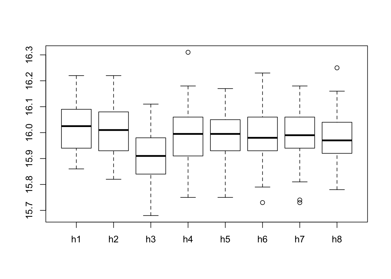
In Chapter Chapter 3 it was proposed to use box plots in order to identify points that are suspected to be outliers. We can use the expression “boxplot(QC$h1)” in order to obtain the box plot of the data of the first hour and go through the names of the variable one by one in order to screen all variable. Alternatively, we may apply the function “boxplot” directly to the data frame “QC” and get a plot with box plots of all the variables in the data frame plotted side by side:

🔗

boxplot(QC)

Box plots for 8 hours of quality control measurements showing potential outliers in hours 4, 6, 7, and 8 — Figure 8.3.5. Box plots for QC data showing potential outliers
🔗

Examining the plots we may see that evidence for the existence of outliers can be spotted on the 4th, 6th, 7th, and 8th hours, providing an answer to Question 4.5

🔗

Example 8.3.6. Estimating the Uniform Distribution Parameter.

A measurement follows the $\text{Uniform}(0,b)\text{,}$ for an unknown value of $b\text{.}$ Two statisticians propose two distinct ways to estimate the unknown quantity $b$ with the aid of a sample of size $n=100\text{.}$ Statistician A proposes to use twice the sample average ($2 \bar X$) as an estimate. Statistician B proposes to use the largest observation instead.

🔗

The motivation for the proposal made by Statistician A is that the expectation of the measurement is equal to $\mathbb{E}(X) = b/2\text{.}$ A reasonable way to estimate the expectation is to use the sample average $\bar X\text{.}$ Thereby, a reasonable way to estimate $b\text{,}$ twice the expectation, is to use $2 \bar X\text{.}$ A motivation for the proposal made by Statistician B is that although the largest observation is indeed smaller that $b\text{,}$ still it may not be much smaller than that value.

🔗

In order to choose between the two options they agreed to prefer the statistic that tends to have values that are closer to $b$ (with respect to the sampling distribution). They also agreed to compute the expectation and variance of each statistic. The performance of a statistic is evaluated using the mean square error (MSE), which is defined as the sum of the variance and the squared difference between the expectation and $b\text{.}$ Namely, if $T$ is the statistic (either the one proposed by Statistician A or Statistician B) then

🔗

\begin{equation*} MSE = \text{Var}(T) + (\mathbb{E}(T) - b)^2\;. \end{equation*}

A smaller mean square error corresponds to a better, more accurate, statistic.

🔗

Assume that the actual value of $b$ is 10 ($b=10$). Use simulations to compute the expectation, the variance and the MSE of the statistic proposed by Statistician A.
🔗

🔗
Assume that the actual value of $b$ is 10 ($b=10$). Use simulations to compute the expectation, the variance and the MSE of the statistic proposed by Statistician B. (Hint: the maximal value of a sequence can be computed with the function “max”.)
🔗

🔗
Assume that the actual value of $b$ is 13.7 ($b=13.7$). Use simulations to compute the expectation, the variance and the MSE of the statistic proposed by Statistician A.
🔗

🔗
Assume that the actual value of $b$ is 13.7 ($b=13.7$). Use simulations to compute the expectation, the variance and the MSE of the statistic proposed by Statistician B. (Hint: the maximal value of a sequence can be computed with the function “max”.)
🔗

🔗
Based on the results in Questions 5.1–4, which of the two statistics seems to be preferable?
🔗

🔗

Solution.

In Questions 5.1 and 5.2 we take the value of $b$ to be equal to 10. Consequently, the distribution of a measurement is $\text{Uniform}(0,10)\text{.}$ In order to generate the sampling distributions we produce two sequences, “A” and “B”, both of length 100,000, with the evaluations of the statistics:

🔗

A <- rep(0,10^5)
B <- rep(0,10^5)
for(i in 1:10^5) {
  X.samp <- runif(100,0,10)
  A[i] <- 2*mean(X.samp)
  B[i] <- max(X.samp)
}

Observe that in each iteration of the “for” loop a sample of size $n=100$ from the $\text{Uniform}(0,10)$ distribution is generated. The statistic proposed by Statistician A (“2*mean(X.samp)”) is computed and stored in sequence “A” and the statistic proposed by Statistician B (“max(X.samp)”) is computed and stored in sequence “B”.

🔗

Consider the statistic proposed by Statistician A:

🔗

mean(A)
var(A)
var(A) + (mean(A)-10)^2

## [1] 9.99772
## [1] 0.3341673
## [1] 0.3341725

The expectation of the statistic is 9.99772 and the variance is 0.3341673. Consequently, we get that the mean square error is equal to

🔗

\begin{equation*} 0.3341673 + (9.99772 - 10)^2 = 0.3341725\;. \end{equation*}

Next, deal with the statistic proposed by Statistician B:

🔗

mean(B)
var(B)
var(B) + (mean(B)-10)^2

## [1] 9.901259
## [1] 0.00950006
## [1] 0.01924989

The expectation of the statistic is 9.901259 and the variance is 0.00950006. Consequently, we get that the mean square error is equal to

🔗

\begin{equation*} 0.00950006 + (9.901259 - 10)^2 = 0.01924989\;. \end{equation*}

Observe that the mean square error of the statistic proposed by Statistician B is smaller.

🔗

For Questions 5.3 and 5.4 we run the same type of simulations. All we change is the value of $b$ (from 10 to 13.7):

🔗

A <- rep(0,10^5)
B <- rep(0,10^5)
for(i in 1:10^5) {
  X.samp <- runif(100,0,13.7)
  A[i] <- 2*mean(X.samp)
  B[i] <- max(X.samp)
}

Again, considering the statistic proposed by Statistician A we get:

🔗

mean(A)
var(A)
var(A) + (mean(A)-13.7)^2

## [1] 13.70009
## [1] 0.6264204
## [1] 0.6264204

The expectation of the statistic in this setting is 13.70009 and the variance is 0.6264204. Consequently, we get that the mean square error is equal to

🔗

\begin{equation*} 0.6264204 + (13.70009 - 13.7)^2 = 0.6264204\;. \end{equation*}

For the statistic proposed by Statistician B we obtain:

🔗

mean(B)
var(B)
var(B) + (mean(B)-13.7)^2

## [1] 13.56467
## [1] 0.01787562
## [1] 0.03618937

The expectation of the statistic is 13.56467 and the variance is 0.01787562. Consequently, we get that the mean square error is equal to

🔗

\begin{equation*} 0.01787562 + (13.56467 - 13.7)^2 = 0.03618937\;. \end{equation*}

Once more, the mean square error of the statistic proposed by Statistician B is smaller.

🔗

Considering the fact that the mean square error of the statistic proposed by Statistician B is smaller in both cases we may conclude that this statistic seems to be better for estimation of $b$ in this setting of Uniformly distributed measurements

As a matter of fact, it can be proved that the statistic proposed by Statistician B has a smaller mean square error than the statistic proposed by Statistician A, for any value of $b$

🔗

Prev Top Next