Section 11.3 Intervals for Normal Measurements
In the construction of the confidence intervals in the previous section it was assumed that the sample size is large enough. This assumption was used both in the application of the Central Limit Theorem and in the substitution of the unknown variance by its estimated value. For a small sample size the reasoning that was applied before may no longer be valid. The Normal distribution may not be a good enough approximation of the sampling distribution of the sample average and the sample variance may differ substantially from the actual value of the measurement variance.
In general, making inference based on small samples requires more detailed modeling of the distribution of the measurements. In this section we will make the assumption that the distribution of the measurements is Normal. This assumption may not fit all scenarios. For example, the Normal distribution is a poor model for the price of a car, which is better modeled by the Exponential distribution. Hence, a blind application of the methods developed in this section to variables such as the price when the sample size is small may produce dubious outcomes and is not recommended.
When the distribution of the measurements is Normal then the method discussed in this section will produce valid confidence intervals for the expectation of the measurement even for a small sample size. Furthermore, we will extend the methodology to enable the construction of confidence intervals for the variance of the measurement.
Before going into the details of the methods let us present an example of inference that involves a small sample. Consider the issue of fuel consumption. Two variables in the “
cars" data frame describe the fuel consumption. The first, “city.mpg", reports the number of miles per gallon when the car is driven in urban conditions and the second, “highway.mpg", reports the miles per gallon in highway conditions. Typically, driving in city conditions requires more stopping and change of speed and is less efficient in terms of fuel consumption. Hence, one expects to obtained a reduced number of miles per gallon when driving in urban conditions compared to the number when driving in highway conditions.
For each car type we calculate the difference variable that measures the difference between the number of miles per gallon in highway conditions and the number in urban conditions. The cars are sub-divided between cars that run on diesel and cars that run on gas. Our concern is to estimate, for each fuel type, the expectation of difference variable and to estimate the variance of that variable. In particular, we are interested in the construction of a confidence intervals for the expectation and a confidence interval for the variance.
Box plots of the difference in fuel consumption between highway and urban conditions are presented in Figure Figure 11.3.1. The box plot on the left hand side corresponds to cars that run on diesel and the box plot on the right hand side corresponds to cars that run on gas. Recall that 20 of the 205 car types use diesel and the other 185 car types use gas. One may suspect that the fuel consumption characteristics vary between the two types of fuel. Indeed, the measurement tends to have sightly higher values for vehicles that use gas.
cars$dif.mpg =  cars$highway.mpg - cars$city.mpg
boxplot(dif.mpg ~ fuel.type, data=cars)
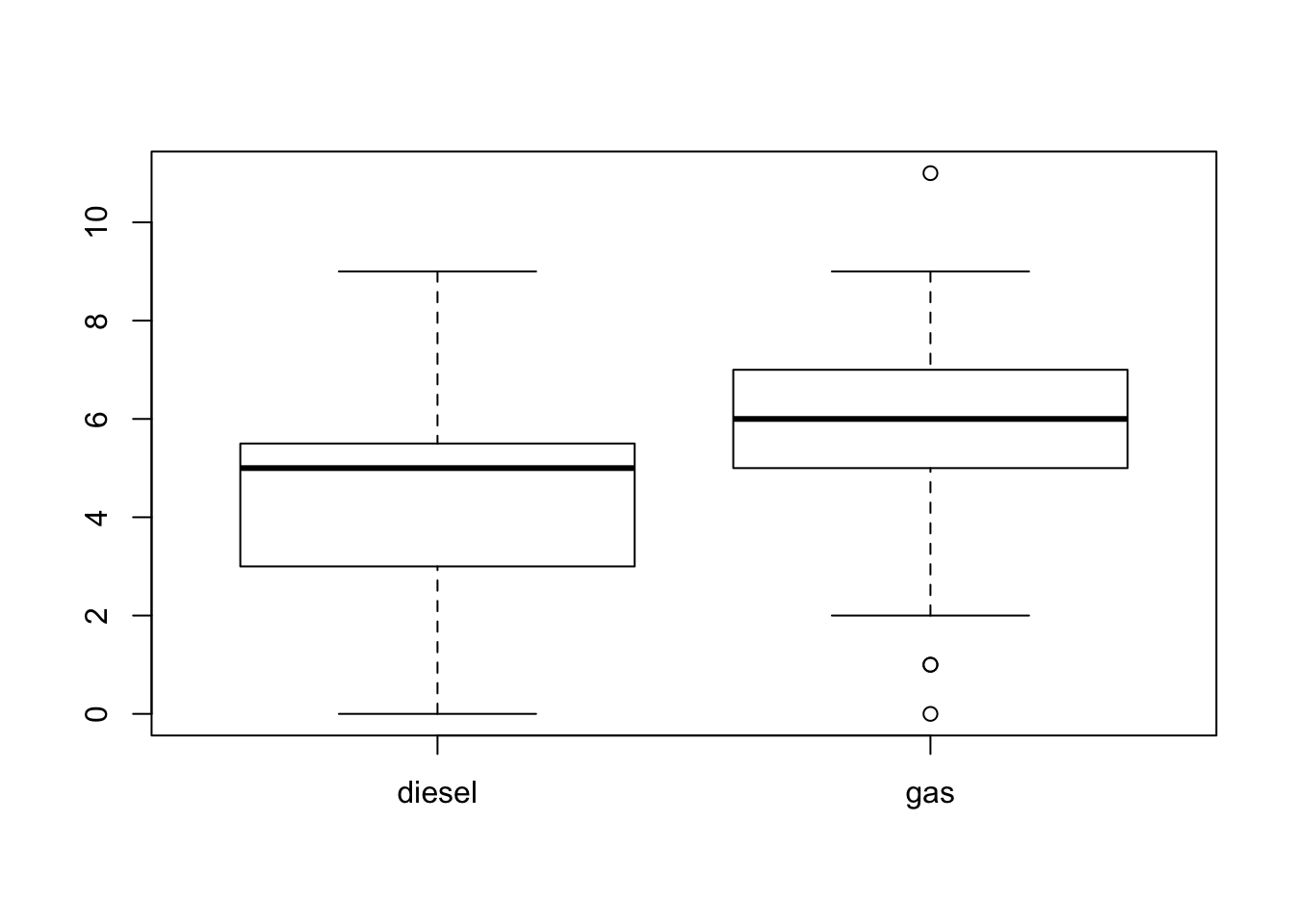
We conduct inference for each fuel type separately. However, since the sample size for cars that run on diesel is only 20, one may have concerns regarding the application of methods that assume a large sample size to a sample size this small.
Subsection 11.3.1 Confidence Intervals for a Normal Mean
Consider the construction of a confidence interval for the expectation of a Normal measurement. In the previous section, when dealing with the construction of a confidence interval for the expectation, we exploited the Central Limit Theorem in order to identify that the distribution of the standardized sample average \((\bar X - \Expec(X))/\sqrt{\Var(X)/n}\) is, approximately, standard Normal. Afterwards, we substituted the standard deviation of the measurement by the sample standard deviation \(S\text{,}\) which was an accurate estimator of the former due to the magnitude sample size.
In the case where the measurements themselves are Normally distributed one can identify the exact distribution of the standardized sample average, with the sample variance substituting the variance of the measurement: \((\bar X - \Expec(X))/(S/\sqrt{n})\text{.}\) This specific distribution is called the Student’s \(t\)-distribution, or simply the \(t\)-distribution.
The \(t\)-distribution is bell shaped and symmetric. Overall, it looks like the standard Normal distribution but it has wider tails. The \(t\)-distribution is characterized by a parameter called the number of degrees of freedom. In the current setting, where we deal with the standardized sample average (with the sample variance substituting the variance of the measurement) the number of degrees of freedom equals the number of observations associated with the estimation of the variance, minus 1. Hence, if the sample size is \(n\) and if the measurement is Normally distributed then the standardized sample average (with \(S\) substituting the standard deviation of the measurement) has a \(t\)-distribution on \((n-1)\) degrees of freedom. We use \(t_{(n-1)}\) to denote this \(t\)-distribution.
The
R system contains functions for the computation of the density, the cumulative probability function and the percentiles of the \(t\)-distribution, as well as for the simulation of a random sample from this distribution. Specifically, the function “qt" computes the percentiles of the \(t\)-distribution. The first argument to the function is a probability and the second argument is the number of degrees of freedom. The output of the function is the percentile associated with the probability of the first argument. Namely, it is a value such that the probability that the \(t\)-distribution is below the value is equal to the probability in the first argument.
For example, let “
n" be the sample size. The output of the expression “qt(0.975,n-1)" is the 0.975-percentile of the \(t\)-distribution on \((n-1)\) degrees of freedom. By definition, 97.5% of the \(t\)-distribution are below this value and 2.5% are above it. The symmetry of the \(t\) distribution implies that 2.5% of the distribution is below the negative of this value. The middle part of the distribution is bracketed by these two values: \([-\mbox{\texttt{qt(0.975,n-1)}}, \mbox{\texttt{qt(0.975,n-1)}}]\text{,}\) and it contains 95% of the distribution.
Summarizing the above claims in a single formula produces the statement:
\begin{equation*}
\frac{\bar X - \Expec(X)}{S/\sqrt{n}} \sim t_{(n-1)} \quad \Longrightarrow \quad \Prob \bigg(\bigg|\frac{\bar X - \Expec(X)}{S/\sqrt{n}}\bigg| \leq \mbox{\texttt{qt(0.975,n-1)}} \bigg) = 0.95\;.
\end{equation*}
Notice that the equation associated with the probability is not an approximation but an exact relation. Rewriting the event that is described in the probability in the form of a confidence interval, produces
1
When the measurement is Normally distributed.
\begin{equation*}
\bar X \pm \mbox{\texttt{qt(0.975,n-1)}}\cdot S/ \sqrt{n}
\end{equation*}
as a confidence interval for the expectation of the Normal measurement with a confidence level of 95%.
The structure of the confidence interval for the expectation of a Normal measurement is essentially identical to the structure proposed in the previous section. The only difference is that the number 1.96, the percentile of the standard Normal distribution, is substituted by the percentile of the \(t\)-distribution.
Consider the construction of a confidence interval for the expected difference in fuel consumption between highway and urban driving conditions. In order to save writing we created two new variables; a factor called “
fuel" that contains the data on the fuel type of each car, and a numerical vector called “dif.mpg" that contains the difference between highway and city fuel consumption for each car type:
fuel <- cars$fuel.type
dif.mpg <- cars$highway.mpg - cars$city.mpg
We are interested in confidence intervals based on the data stored in the variable “
dif.mpg". One confidence interval will be associated with the level “diesel" of the factor “fuel" and the other will be associated with the level “gas" of the same factor.
In order to compute these confidence intervals we need to compute, for each level of the factor “
fuel", the sample average and the sample standard deviation of the data points of the variable “dif.mpg" that are associated with that level.
It is convenient to use the function “
tapply" for this task. This function uses three arguments. The first argument is the sequence of values over which we want to carry out some computation. The second argument is a factor. The third argument is a name of a function that is used for the computation. The function “tapply" applies the function in the third argument to each sub-collection of values of the first argument. The sub-collections are determined by the levels of the second argument.
Sounds complex but it is straightforward enough to apply:
tapply(dif.mpg,fuel,mean)
tapply(dif.mpg,fuel,sd)
##   diesel      gas
## 4.450000 5.648649
##   diesel      gas
## 2.781045 1.433607
Sample averages are computed in the first application of the function “
tapply". Observe that an average was computed for cars that run on diesel and an average was computed for cars that run on gas. In both cases the average corresponds to the difference in fuel consumption. Similarly, the standard deviations were computed in the second application of the function. We obtain that the point estimates of the expectation for diesel and gas cars are 4.45 and 5.648649, respectively and the point estimates for the standard deviation of the variable are 2.781045 and 1.433607.
Let us compute the confidence interval for each type of fuel:
x.bar <- tapply(dif.mpg,fuel,mean)
s <- tapply(dif.mpg,fuel,sd)
n <- c(20,185)
x.bar - qt(0.975,n-1)*s/sqrt(n)
x.bar + qt(0.975,n-1)*s/sqrt(n)
##   diesel      gas
## 3.148431 5.440699
##   diesel      gas
## 5.751569 5.856598
The objects “
x.bar" and “s" contain the sample averages and sample standard deviations, respectively. Both are sequences of length two, with the first component referring to “diesel" and the second component referring to “gas". The object “n" contains the two sample sizes, 20 for “diesel" and 185 for “gas". In the expression next to last the lower boundary for each of the confidence intervals is computed and in the last expression the upper boundary is computed. The confidence interval for the expected difference in diesel cars is \([3.148431, 5.751569]\text{.}\) and the confidence interval for cars using gas is \([5.440699, 5.856598]\text{.}\)
The 0.975-percentiles of the \(t\)-distributions are computed with the expressions “
qt(0.025,n-1)":
qt(0.975,n-1)
## [1] 2.093024 1.972941
The second argument of the function “
qt" is a sequence with two components, the number 19 and the number 184. Accordingly, The first position in the output of the function is the percentile associated with 19 degrees of freedom and the second position is the percentile associated to 184 degrees of freedom.
Compare the resulting percentiles to the 0.975-percentile of the standard Normal distribution, which is essentially equal to 1.96. When the sample size is small, 20 for example, the percentile of the \(t\)-distribution is noticeably larger than the percentile of the standard Normal. However, for a larger sample size the percentiles, more or less, coincide. It follows that for a large sample the method proposed in Subsection 11.2.2 and the method discussed in this subsection produce essentially the same confidence intervals.
Subsection 11.3.2 Confidence Intervals for a Normal Variance
The next task is to compute confidence intervals for the variance of a Normal measurement. The main idea in the construction of a confidence interval is to identify the distribution of a random variable associated with the parameter of interest. A region that contains 95% of the distribution of the random variable (or, more generally, the central part of the distribution of probability equal to the confidence level) is identified. The confidence interval results from the reformulation of the event associated with that region. The new formulation puts the parameter between a lower limit and an upper limit. These lower and the upper limits are computed from the data and they form the boundaries of the confidence interval.
We start with the sample variance, \(S^2 = \sum_{i=1}^n (X_i - \bar X)^2/(n-1)\text{,}\) which serves as a point estimator of the parameter of interest. When the measurements are Normally distributed then the random variable \((n-1)S^2/\sigma^2\) possesses a special distribution called the chi-square distribution. (Chi is the Greek letter \(\chi\text{,}\) which is read “Kai".) This distribution is associated with the sum of squares of Normal variables. It is parameterized, just like the \(t\)-distribution, by a parameter called the number of degrees of freedom. This number is equal to \((n-1)\) in the situation we discuss. The chi-square distribution on \((n-1)\) degrees of freedom is denoted with the symbol \(\chi^2_{(n-1)}\text{.}\)
The
R system contains functions for the computation of the density, the cumulative probability function and the percentiles of the chi-square distribution, as well as for the simulation of a random sample from this distribution. Specifically, the percentiles of the chi-square distribution are computed with the aid of the function “qchisq". The first argument to the function is a probability and the second argument is the number of degrees of freedom. The output of the function is the percentile associated with the probability of the first argument. Namely, it is a value such that the probability that the chi-square distribution is below the value is equal to the probability in the first argument.
For example, let “
n" be the sample size. The output of the expression “qt(0.975,n-1)" is the 0.975-percentile of the chi-square distribution. By definition, 97.5% of the chi-square distribution are below this value and 2.5% are above it. Similarly, the expression “qchisq(0.025,n-1)" is the 0.025-percentile of the chi-square distribution, with 2.5% of the distribution below this value. Notice that between these two percentiles, namely within the interval \([\mbox{\texttt{qchisq(0.025,n-1)}}, \mbox{\texttt{qchisq(0.975,n-1)}}]\text{,}\) are 95% of the chi-square distribution.
We may summarize that for Normal measurements:
\begin{equation*}
\begin{aligned}
\lefteqn{(n-1)S^2/\sigma^2 \sim \chi^2_{(n-1)} \quad \Longrightarrow }\\ & \Prob \big( \mbox{\texttt{qchisq(0.025,n-1)}} \leq (n-1)S^2/\sigma^2 \leq \mbox{\texttt{qchisq(0.975,n-1)}} \big) = 0.95\;.\end{aligned}
\end{equation*}
The chi-square distribution is not symmetric. Therefore, in order to identify the region that contains 95% of the distribution region we have to compute both the 0.025- and the 0.975-percentiles of the distribution.
The event associated with the 95% region is rewritten in a form that puts the parameter \(\sigma^2\) in the center:
\begin{equation*}
\big\{(n-1)S^2/\mbox{\texttt{qchisq(0.975,n-1)}} \leq \sigma^2 \leq (n-1)S^2/\mbox{\texttt{qchisq(0.025,n-1)}}\big\}\;.
\end{equation*}
The left most and the right most expressions in this event mark the end points of the confidence interval. The structure of the confidence interval is:
\begin{equation*}
\big[\{(n-1)/\mbox{\texttt{qchisq(0.975,n-1)}}\}\times S^2,\;\{(n-1)/\mbox{\texttt{qchisq(0.025,n-1)}}\}\times S^2\big]\;.
\end{equation*}
Consequently, the confidence interval is obtained by the multiplication of the estimator of the variance by a ratio between the number of degrees of freedom (\(n-1\)) and an appropriate percentile of the chi-square distribution. The percentile on the left hand side is associated with the larger probability (making the ratio smaller) and the percentile on the right hand side is associated with the smaller probability (making the ratio larger).
Consider, specifically, the confidence intervals for the variance of the measurement “
diff.mpg" for cars that run on diesel and for cars that run on gas. Here, the size of the samples is 20 and 185, respectively:
(n-1)/qchisq(0.975,n-1)
(n-1)/qchisq(0.025,n-1)
## [1] 0.5783456 0.8234295
## [1] 2.133270 1.240478
The ratios that are used in the left hand side of the intervals are 0.5783456 and 0.8234295, respectively. Both ratios are less than one. On the other hand, the ratios associated with the other end of the intervals, 2.133270 and 1.240478, are both larger than one.
Let us compute the point estimates of the variance and the associated confidence intervals. Recall that the object “
s" contains the sample standard deviations of the difference in fuel consumption for diesel and for gas cars. The object “n" contains the two sample sizes:
s^2
(n-1)*s^2/qchisq(0.975,n-1)
(n-1)*s^2/qchisq(0.025,n-1)
##   diesel      gas
## 7.734211 2.055229
##   diesel      gas
## 4.473047 1.692336
##   diesel      gas
## 16.499155  2.549466
The variance of the difference in fuel consumption for diesel cars is estimated to be 7.734211 with a 95%-confidence interval of \([4.473047, 16.499155]\) and for cars that use gas the estimated variance is 2.055229, with a confidence interval of \([1.692336, 2.549466]\text{.}\)
As a final example in this section let us simulate the confidence level for a confidence interval for the expectation and for a confidence interval for the variance of a Normal measurement. In this simulation we assume that the expectation is equal to \(\mu = 3\) and the variance is equal to \(\sigma^2 = 3^2 = 9\text{.}\) The sample size is taken to be \(n=20\text{.}\) We start by producing the sampling distribution of the sample average \(\bar X\) and of the sample standard deviation \(S\text{:}\)
mu <- 4
sig <- 3
n <- 20
X.bar <- rep(0,10^5)
S <- rep(0,10^5)
for(i in 1:10^5) {
  X <- rnorm(n,mu,sig)
  X.bar[i] <- mean(X)
  S[i] <- sd(X)
}
Consider first the confidence interval for the expectation:
mu.LCL <- X.bar - qt(0.975,n-1)*S/sqrt(n)
mu.UCL <- X.bar + qt(0.975,n-1)*S/sqrt(n)
mean((mu >= mu.LCL) & (mu <= mu.UCL))
## [1] 0.95009
The nominal significance level of the confidence interval is 95%, which is practically identical to the confidence level that was computed in the simulation.
The confidence interval for the variance is obtained in a similar way. The only difference is that we apply now different formulae for the computation of the upper and lower confidence limits:
var.LCL <- (n-1)*S^2/qchisq(0.975,n-1)
var.UCL <- (n-1)*S^2/qchisq(0.025,n-1)
mean((sig^2 >= var.LCL) & (sig^2 <= var.UCL))
## [1] 0.94959
Again, we obtain that the nominal confidence level of 95% coincides with the confidence level computed in the simulation.

