Section 15.3 Logistic Regression
In the previous section we considered a Bernoulli response and a factor with two levels as an explanatory variable. In this section we use a numeric variable as the explanatory variable. The discussion in this section is parallel to the discussion in Chapter 14 that presented the topic of linear regression. However, since the response is not of the same form, it is the indicator of a level of a factor and not a regular numeric response, then the tools the are used are different. Instead of using linear regression we use another type of regression that is called Logistic Regression.
Recall that linear regression involved fitting a straight line to the scatter plot of data points. This line corresponds to the expectation of the response as a function of the explanatory variable. The estimated coefficients of this line are computed from the data and used for inference.
In logistic regression, instead of the consideration of the expectation of a numerical response, one considers the probability of an event associated with the response. This probability is treated as a function of the explanatory variable. Parameters that determine this function are estimated from the data and are used for inference regarding the relation between the explanatory variable and the response. Again, we do not discuss the theoretical details involved in the derivation of logistic regression. Instead, we apply the method to an example.
We consider the factor
num.of.doors as the response and the probability of a car with four doors as the probability of the response. The length of the car will serve as the explanatory variable. Measurements of lengths of the cars are stored in the variable length in the data frame cars.
First, let us plot the relation between the response and the explanatory variable:
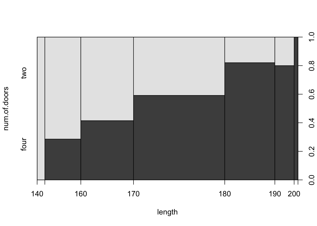
plot(num.of.doors ~ length,data=cars)
The plot is a type of a mosaic plot and it is produced when the input to the function
plot is a formula with a factor as a response and a numeric variable as the explanatory variable. The plot presents, for interval levels of the explanatory variable, the relative frequencies of each interval. It also presents the relative frequency of the levels of the response within each interval level of the explanatory variable.
In order to get a better understanding of the meaning of the given mosaic plot one may consider the histogram of the explanatory variable.
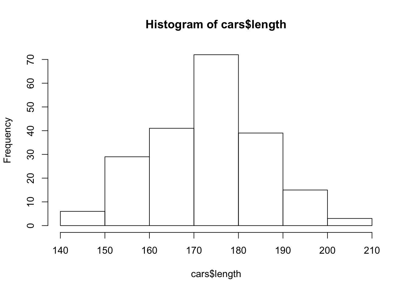
hist(cars$length)
The histogram involves the partition of the range of variable length into intervals. These interval are the basis for rectangles. The height of the rectangles represent the frequency of cars with lengths that fall in the given interval.
The mosaic plot in Figure 15.3.1 is constructed on the basis of this histogram. The \(x\)-axis in this plot corresponds to the explanatory variable
length. The total area of the square in the plot is divided between 7 vertical rectangles. These vertical rectangles correspond to the 7 rectangles in the histogram of Figure 15.3.2, turn on their sides. Hence, the width of each rectangle in Figure 15.3.1 correspond to the height of the parallel rectangle in the histogram. Consequently, the area of the vertical rectangles in the mosaic plot represents the relative frequency of the associated interval of values of the explanatory variable.
The rectangle that is associated with each interval of values of the explanatory variable is further divided into horizontal sub-rectangles that are associated with the response factor. In the current example each darker rectangle is associated with the level
four of the response num.of.door and each brighter rectangle is associated with the level two. The relative area of the horizontal rectangles within each vertical rectangle represent the relative frequency of the levels of the response within each interval of values of the explanatory variable.
From the examination of the mosaic plot one may identify relations between the explanatory variable and the relative frequency of an identified level of the response. In the current example one may observe that the relative frequency of the cars with four doors is, overall, increasing with the increase in the length of cars.
Logistic regression is a method for the investigation of relations between the probability of an event and explanatory variables. Specifically, we use it here for making inference on the number of doors as a response and the length of the car as the explanatory variable.
Statistical inference requires a statistical model. The statistical model in logistic regression relates the probability \(p_i\text{,}\) the probability of the event for observation \(i\text{,}\) to \(x_i\text{,}\) the value of the response for that observation. The relation between the two in given by the formula:
\begin{equation*}
p_i = \frac{e^{a + b \cdot x_i}}{1 + e^{a + b\cdot x_i}}\;,
\end{equation*}
where \(a\) and \(b\) are coefficients common to all observations. Equivalently, one may write the same relation in the form:
\begin{equation*}
\log(p_i/[1-p_i]) = a + b\cdot x_i\;,
\end{equation*}
that states that the relation between a (function of) the probability of the event and the explanatory variable is a linear trend.
One may fit the logistic regression to the data and test the null hypothesis by the use of the function
glm:
fit.doors <- glm(num.of.doors=="four"~length, family=binomial,data=cars)
summary(fit.doors)
##
## Call:
## glm(formula = num.of.doors == "four" ~ length, family = binomial,
##     data = cars)
##
## Deviance Residuals:
##     Min       1Q   Median       3Q      Max
## -2.4301  -0.8314   0.2899   0.8024   1.8839
##
## Coefficients:
##              Estimate Std. Error z value Pr(>|z|)
## (Intercept) -13.14767    2.70089  -4.868 1.13e-06 ***
## length        0.07726    0.01559   4.955 7.20e-07 ***
## ---
## Signif. codes:  0 '***' 0.001 '**' 0.01 '*' 0.05 '.' 0.1 ' ' 1
##
## (Dispersion parameter for binomial family taken to be 1)
##
##     Null deviance: 281.40  on 202  degrees of freedom
## Residual deviance: 237.28  on 201  degrees of freedom
## AIC: 241.28
##
## Number of Fisher Scoring iterations: 4
Generally, the function . Alternatively, it may be a sequence with “1” or “0” values, “1” corresponding to the event occurring to the subject and “0” corresponding to the event not occurring. The argument
glm can be used in order to fit regression models in cases where the distribution of the response has special forms. Specifically, when the argument family=binomial is used then the model that is being used is the logistic regression model. The formula that is used in the function involves a response and an explanatory variable. The response may be a sequence with logical TRUE or FALSE values as in the example1
The response is the output of the expression
num.of.doors==four. This expression produces logical values. TRUE when the car has 4 doors and FALSE when it has 2 doors.
data=cars is used in order to inform the function that the variables are located in the given data frame.
A report is produced when the function
summary is applied to the fitted model. Notice the similarities and the differences between the report presented here and the reports for linear regression that are presented in Chapter 14. Both reports contain estimates of the coefficients \(a\) and \(b\) and tests for the equality of these coefficients to zero. When the coefficient \(b\text{,}\) the coefficient that represents the slope, is equal to 0 then the probability of the event and the explanatory variable are unrelated. In the current case we may note that the null hypothesis \(H_0: b = 0\text{,}\) the hypothesis that claims that there is no relation between the explanatory variable and the response, is clearly rejected (\(p\)-value \(2.37 \times 10^{-7}\)).
The estimated values of the coefficients are \(-13.14767\) for the intercept \(a\) and \(0.07726\) for the slope \(b\text{.}\) One may produce confidence intervals for these coefficients by the application of the function
confint to the fitted model:
confint(fit.doors)
## Waiting for profiling to be done...
##                   2.5 %      97.5 %
## (Intercept) -18.8530894 -8.05800914
## length        0.0479835  0.10948463

