Introduction to Statistical Thinking

The relation between the random sample and the data is similar to the relation between a random variable and the observed value. The data is the observed values of a sample taken from a population. The content of the data is known. The random sample, similarly to a random variable, is the data that will be selected when taking a sample, prior to the selection itself. The content of the random sample is unknown, since the sample has not yet been taken. Still, just like for the case of the random variable, one is able to say what the possible evaluations of the sample may be and, depending on the mechanism of selecting the sample, what are the probabilities of the different potential evaluations. The collection of all possible evaluations of the sample is the sample space of the random sample and the probabilities of the different evaluations produce the distribution of the random sample.

(Alternatively, if one prefers to speak in past tense, one can define the sample space of a random sample to be the evaluations of the sample that could have taken place, with the distribution of the random sample being the probabilities of these evaluations.)

A statistic is a function of the data. Example of statistics are the average of the data, the sample variance and standard deviation, the median of the data, etc. In each case a given formula is applied to the data. In each type of statistic a different formula is applied.

The same formula that is applied to the observed data may, in principle, be applied to random samples. Hence, for example, one may talk of the sample average, which is the average of the elements in the data. The average, considered in the context of the observed data, is a number and its value is known. However, if we think of the average in the context of a random sample then it becomes a random variable. Prior to the selection of the actual sample we do not know what values it will include. Hence, we cannot tell what the outcome of the average of the values will be. However, due to the identification of all possible evaluations that the sample can possess we may say in advance what is the collection of values the sample average can have. This is the sample space of the sample average. Moreover, from the sampling distribution of the random sample one may identify the probability of each value of the sample average, thus obtaining the sampling distribution of the sample average.

The same line of argumentation applies to any statistic. Computed in the context of the observed data, the statistic is a known number that may, for example, be used to characterize the variation in the data. When thinking of a statistic in the context of a random sample it becomes a random variable. The distribution of the statistic is called the sampling distribution of the statistic. Consequently, we may talk of the sampling distribution of the median, the sample distribution of the sample variance, etc.

Random variables are also applied as models for uncertainty in future measurements in more abstract settings that need not involve a specific population. Specifically, we introduced the Binomial and Poisson random variables for settings that involve counting and the Uniform, Exponential, and Normal random variables for settings where the measurement is continuous.

The notion of a sampling distribution may be extended to a situation where one is taking several measurements, each measurement taken independently of the others. As a result one obtains a sequence of measurements. We use the term “sample” to denote this sequence. The distribution of this sequence is also called the sampling distribution. If all the measurements in the sequence are Binomial then we call it a Binomial sample. If all the measurements are Exponential we call it an Exponential sample and so forth.

Again, one may apply a formula (such as the average) to the content of the random sequence and produce a random variable. The term sampling distribution describes again the distribution that the random variable produced by the formula inherits from the sample.

In the next subsection we examine an example of a sample taken from a population. Subsequently, we discuss examples that involves a sequence of measurements from a theoretical model.

Consider taking a sample from a population. Let us use again for the illustration the file “pop1.csv” like we did in Chapter 4. The data frame produced from the file contains the sex and height of the 100,000 members of some imaginary population. Recall that in Chapter 4 we applied the function “sample” to randomly sample the height of a single subject from the population. Let us apply the same function again, but this time in order to sample the heights of 100 subjects:

pop.1 <- read.csv("_data/pop1.csv")
X.samp <- sample(pop.1$height,100)
X.samp

##   [1] 178 182 183 172 177 161 163 185 143 157 171 182 182 178 157 165 153
##  [18] 178 164 168 180 166 192 182 172 164 163 182 165 141 157 158 188 168
##  [35] 161 158 160 162 163 170 171 183 173 160 178 171 159 170 190 179 159
##  [52] 173 160 174 179 172 176 181 171 186 155 165 175 191 169 179 166 184
##  [69] 181 166 158 168 165 168 155 185 196 145 153 163 172 163 177 184 165
##  [86] 156 140 202 162 157 176 176 171 166 185 171 184 173 174 162

In the first line of code we produce a data frame that contains the information on the entire population. In the second line we select a sample of size 100 from the population, and in the third line we present the content of the sample.

The first argument to the function “sample” that selects the sample is the sequence of length 100,000 with the list of heights of all the members of the population. The second argument indicates the sample size, 100 in this case. The outcome of the random selection is stored in the object “X.samp”, which is a sequence that contains 100 heights.

Typically, a researcher does not get to examine the entire population. Instead, measurements on a sample from the population are made. In relation to the imaginary setting we simulate in the example, the typical situation is that the research does not have the complete list of potential measurement evaluations, i.e. the complete list of 100,000 heights in “pop.1$height”, but only a sample of measurements, namely the list of 100 numbers that are stored in “X.samp” and are presented above. The role of statistics is to make inference on the parameters of the unobserved population based on the information that is obtained from the sample.

For example, we may be interested in estimating the mean value of the heights in the population. A reasonable proposal is to use the sample average to serve as an estimate:

mean(X.samp)

## [1] 170.19

In our artificial example we can actually compute the true population mean:

mean(pop.1$height)

## [1] 170.035

Hence, we may see that although the match between the estimated value and the actual value is not perfect still they are close enough.

The actual estimate that we have obtained resulted from the specific sample that was collected. Had we collected a different subset of 100 individuals we would have obtained different numerical value for the estimate. Consequently, one may wonder: Was it pure luck that we got such good estimates? How likely is it to get estimates that are close to the target parameter?

Notice that in realistic settings we do not know the actual value of the target population parameters. Nonetheless, we would still want to have at least a probabilistic assessment of the distance between our estimates and the parameters they try to estimate. The sampling distribution is the vehicle that may enable us to address these questions.

In order to illustrate the concept of the sampling distribution let us select another sample and compute its average:

X.samp <- sample(pop.1$height,100)
X.bar <- mean(X.samp)
X.bar

## [1] 169.08

and do it once more:

X.samp <- sample(pop.1$height,100)
X.bar <- mean(X.samp)
X.bar

## [1] 170.89

In each case we got a different value for the sample average. In the first of the last two iterations the result was more than 1 centimeter away from the population average, which is equal to 170.035, and in the second it was within the range of 1 centimeter. Can we say, prior to taking the sample, what is the probability of falling within 1 centimeter of the population mean?

Chapter 4 discussed the random variable that emerges by randomly sampling a single number from the population presented by the sequence “pop.1$height”. The distribution of the random variable resulted from the assignment of the probability 1/100,000 to each one of the 100,000 possible outcomes. The same principle applies when we randomly sample 100 individuals. Each possible outcome is a collection of 100 numbers and each collection is assigned equal probability. The resulting distribution is called the sampling distribution.

The distribution of the average of the sample emerges from this distribution: With each sample one may associate the average of that sample. The probability assigned to that average outcome is the probability of the sample. Hence, one may assess the probability of falling within 1 centimeter of the population mean using the sampling distribution. Each sample produces an average that either falls within the given range or not. The probability of the sample average falling within the given range is the proportion of samples for which this event happens among the entire collection of samples.

However, we face a technical difficulty when we attempt to assess the sampling distribution of the average and the probability of falling within 1 centimeter of the population mean. Examination of the distribution of a sample of a single individual is easy enough. The total number of outcomes, which is 100,000 in the given example, can be handled with no effort by the computer. However, when we consider samples of size 100 we get that the total number of ways to select 100 number out of 100,000 numbers is in the order of \(10^{342}\) (1 followed by 342 zeros) and cannot be handled by any computer. Thus, the probability cannot be computed.

As a compromise we will approximate the distribution by selecting a large number of samples, say 100,000, to represent the entire collection, and use the resulting distribution as an approximation of the sampling distribution. Indeed, the larger the number of samples that we create the more accurate the approximation of the distribution is. Still, taking 100,000 repeats should produce approximations which are good enough for our purposes.

Consider the sampling distribution of the sample average. We simulated above a few examples of the average. Now we would like to simulate 100,000 such examples. We do this by creating first a sequence of the length of the number of evaluations we seek (100,000) and then write a small program that produces each time a new random sample of size 100 and assigns the value of the average of that sample to the appropriate position in the sequence. Do first and explain later

¹

Running this simulation, and similar simulations of the same nature that will be considered in the sequel, demands more of the computer’s resources than the examples that were considered up until now. Beware that running times may be long and, depending on the strength of your computer and your patience, too long. You may save time by running less iterations, replacing, say, “10^5” by “10^4”. The results of the simulation will be less accurate, but will still be meaningful.

:

X.bar <- rep(0,10^5)
for(i in 1:10^5) {
  X.samp <- sample(pop.1$height,100)
  X.bar[i] <- mean(X.samp)
}

In the first line we produce a sequence of length 100,000 that contains zeros. The function “rep” creates a sequence that contains repeats of its first argument a number of times that is specified by its second argument. In this example, the numerical value 0 is repeated 100,000 times to produce a sequence of zeros of the length we seek.

The main part of the program is a “for” loop. The argument of the function “for” takes the special form: “index.name in index.values”, where index.name is the name of the running index and index.values is the collection of values over which the running index is evaluated. In each iteration of the loop the running index is assigned a value from the collection and the expression that follows the brackets of the “for” function is evaluated with the given value of the running index.

In the given example the collection of values is produced by the expression “1:n”. Recall that the expression “1:n” produces the collection of integers between 1 and n. Here, n = 100,000. Hence, in the given application the collection of values is a sequence that contains the integers between 1 and 100,000. The running index is called “i”. the expression is evaluated 100,000 times, each time with a different integer value for the running index “i”.

The R system treats a collection of expressions enclosed within curly brackets as one entity. Therefore, in each iteration of the “for” loop, the lines that are within the curly brackets are evaluated. In the first line a random sample of size 100 is produced and in the second line the average of the sample is computed and stored in the \(i\)-th position of the sequence “X.bar”. Observe that the specific position in the sequence is referred to by using square brackets.

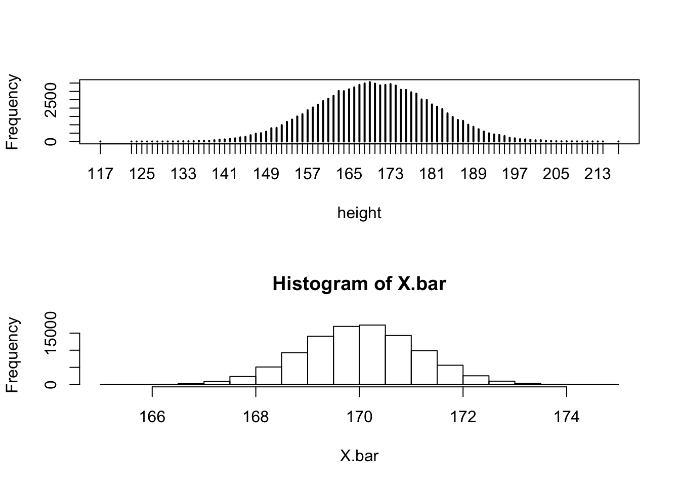
The program changes the original components of the sequence, from 0 to the average of a random sample, one by one. When the loop ends all values are changed and the sequence “X.bar” contains 100,000 evaluations of the sample average. The last line, which is outside the curly brackets and is evaluated after the “for” loop ends, produces an histogram of the averages that were simulated. The histogram is presented in the lower panel of Figure 7.2.1.

Compare the distribution of the sample average to the distribution of the heights in the population that was presented first in Figure 4.3.1 and is currently presented in the upper panel of Figure 7.2.1. Observe that both distributions are centered at about 170 centimeters. Notice, however, that the range of values of the sample average lies essentially between 166 and 174 centimeters, whereas the range of the distribution of heights themselves is between 127 and 217 centimeter. Broadly speaking, the sample average and the original measurement are centered around the same location but the sample average is less spread.

Specifically, let us compare the expectation and standard deviation of the sample average to the expectation and standard deviation of the original measurement:

mean(pop.1$height)
sd(pop.1$height)
mean(X.bar)
sd(X.bar)

## [1] 170.035
## [1] 11.23205
## [1] 170.0346
## [1] 1.11987

Observe that the expectation of the population and the expectation of the sample average are practically the same, but the standard deviation of the sample average is about 10 times smaller than the standard deviation of the population. This result is not accidental and actually reflects a general phenomena that will be seen below in other examples.

We may use the simulated sampling distribution in order to compute an approximation of the probability of the sample average falling within 1 centimeter of the population mean. Let us first compute the relevant probability and then explain the details of the computation:

mean(abs(X.bar - mean(pop.1$height)) <= 1)

## [1] 0.62649

Hence we get that the probability of the given event is about 62.6%.

The object “X.bar” is a sequence of length 100,000 that contains the simulated sample averages. This sequence represents the distribution of the sample average. The expression “abs(X.bar - mean(pop.1$height)) <= 1” produces a sequence of logical “TRUE” or “FALSE” values, depending on the value of the sample average being less or more than one unit away from the population mean. The application of the function “mean” to the output of the last expression results in the computation of the relative frequency of TRUEs, which corresponds to the probability of the event of interest.

Sampling distribution can also be considered in the context of theoretical distribution models. For example, take a measurement \(X \sim \mathrm{Binomial}(10,0.5)\) from the Binomial distribution. Assume 64 independent measurements are produced with this distribution: \(X_1, X_2, \ldots, X_{64}\text{.}\) The sample average in this case corresponds to the distribution of the random variable produced by averaging these 64 random variables:

Again, one may wonder what is the distribution of the sample average \(\bar X\) in this case?

We can approximate the distribution of the sample average by simulation. The function “rbinom” produces a random sample from the Binomial distribution. The first argument to the function is the sample size, which we take in this example to be equal to 64. The second and third arguments are the parameters of the Binomial distribution, 10 and 0.5 in this case. We can use this function in the simulation:

X.bar <- rep(0,10^5)
for(i in 1:10^5) {
  X.samp <- rbinom(64,10,0.5)
  X.bar[i] <- mean(X.samp)
}

Observe that in this code we created a sequence of length 100,000 with evaluations of the sample average of 64 Binomial random variables. We start with a sequence of zeros and in each iteration of the “for” loop a zero is replaced by the average of a random sample of 64 Binomial random variables.

Examine the sampling distribution of the Binomial average:

mean(X.bar)
sd(X.bar)

## [1] 5.000031
## [1] 0.198051

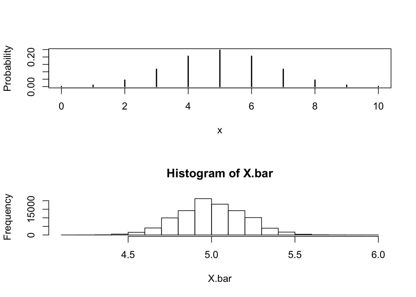
The histogram of the sample average is presented in the lower panel of Figure 7.2.3. Compare it to the distribution of a single Binomial random variable that appears in the upper panel. Notice, once more, that the center of the two distributions coincide but the spread of the sample average is smaller. The sample space of a single Binomial random variable is composed of integers. The sample space of the average of 64 Binomial random variables, on the other hand, contains many more values and is closer to the sample space of a random variable with a continuous distribution.

Recall that the expectation of a \(\mathrm{Binomial}(10,0.5)\) random variable is \(\Expec(X) = 10 \cdot 0.5 = 5\) and the variance is \(\Var(X) = 10 \cdot 0.5 \cdot 0.5 = 2.5\) (thus, the standard deviation is \(\sqrt{2.5} = 1.581139\)). Observe that the expectation of the sample average that we got from the simulation is essentially equal to 5 and the standard deviation is 0.1982219.

One may prove mathematically that the expectation of the sample mean is equal to the theoretical expectation of its components:

The results of the simulation for the expectation of the sample average are consistent with the mathematical statement. The mathematical theory of probability may also be used in order to prove that the variance of the sample average is equal to the variance of each of the components, divided by the sample size:

here \(n\) is the number of observations in the sample. Specifically, in the Binomial example we get that \(\Var(\bar X) = 2.5/64\text{,}\) since the variance of a Binomial component is 2.5 and there are 64 observations. Consequently, the standard deviation is \(\sqrt{2.5/64} = 0.1976424\text{,}\) in agreement, more or less, with the results of the simulation (that produced 0.1982219 as the standard deviation).

Consider the problem of identifying the central interval that contains 95% of the distribution. In the Normal distribution we were able to use the function “qnorm” in order to compute the percentiles of the theoretical distribution. A function that can be used for the same purpose for simulated distribution is the function “quantile”. The first argument to this function is the sequence of simulated values of the statistic, “X.bar” in the current case. The second argument is a number between 0 and 1, or a sequence of such numbers:

quantile(X.bar,c(0.025,0.975))

##     2.5%    97.5% 
## 4.609375 5.390625

We used the sequence “c(0.025,0.975)” as the input to the second argument. As a result we obtained the output 4.609375, which is the 2.5%-percentile of the sampling distribution of the average, and 5.390625, which is the 97.5%-percentile of the sampling distribution of the average.

Of interest is to compare these percentiles to the parallel percentiles of the Normal distribution with the same expectation and the same standard deviation as the average of the Binomials:

qnorm(c(0.025,0.975),mean(X.bar),sd(X.bar))

## [1] 4.611859 5.388204

Observe the similarity between the percentiles of the distribution of the average and the percentiles of the Normal distribution. This similarity is a reflection of the Normal approximation of the sampling distribution of the average, which is formulated in the next section under the title: The Central Limit Theorem.