Introduction to Statistical Thinking

A particular measles vaccine produces a reaction (a fever higher that 102 Fahrenheit) in each vaccinee with probability of 0.09. A clinic vaccinates 500 people each day.

1. What is the expected number of people that will develop a reaction each day?

2. What is the standard deviation of the number of people that will develop a reaction each day?

3. In a given day, what is the probability that more than 40 people will develop a reaction?

4. In a given day, what is the probability that the number of people that will develop a reaction is between 50 and 45 (inclusive)?

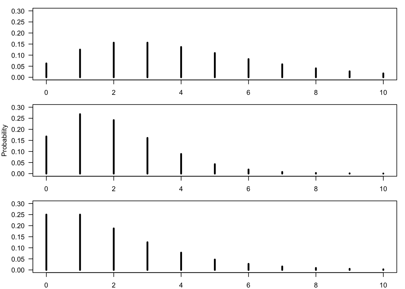
The Negative-Binomial distribution is yet another example of a discrete, integer valued, random variable. The sample space of the distribution are all non-negative integers \(\{0, 1, 2, \ldots\}\text{.}\) The fact that a random variable \(X\) has this distribution is marked by “\(X \sim \mbox{Negative-Binomial}(r,p)\)", where \(r\) and \(p\) are parameters that specify the distribution.

Consider 3 random variables from the Negative-Binomial distribution:

The bar plots of these random variables are presented in Figure 5.4.2, reorganized in a random order.

1. Produce bar plots of the distributions of the random variables \(X_1\text{,}\) \(X_2\text{,}\) \(X_3\) in the range of integers between 0 and 15 and thereby identify the pair of parameters that produced each one of the plots in Figure 5.4.2. Notice that the bar plots can be produced with the aid of the function “plot" and the function “dnbinom(x,r,p)", where “x" is a sequence of integers and “r" and “p" are the parameters of the distribution. Pay attention to the fact that you should use the argument “type = h" in the function “plot" in order to produce the horizontal bars.

2. Below is a list of pairs that includes an expectation and a variance. Each of the pairs is associated with one of the random variables \(X_1\text{,}\) \(X_2\text{,}\) and \(X_3\text{:}\)

1. \(\Expec(X) = 4\text{,}\) \(\Var(X) = 8\text{.}\)

2. \(\Expec(X) = 2\text{,}\) \(\Var(X) = 4\text{.}\)

3. \(\Expec(X) = 2\text{,}\) \(\Var(X) = 2.5\text{.}\)

Use Figure 5.4.2 in order to match the random variable with its associated pair. Do not use numerical computations or formulae for the expectation and the variance in the Negative-Binomial distribution in order to carry out the matching

¹

It can be shown, or else found on the web, that if \(X\sim \mbox{Negative-Binomial}(r,p)\) then \(\Expec(X) = r(1-p)/p\) and \(\Var(X) = r(1-p)/p^2\text{.}\)

. Use, instead, the structure of the bar-plots.