Section 14.4 R-squared and the Variance of Residuals
In this section we discuss the residuals between the values of the response and their estimated expected value according to the regression model. These residuals are the regression model equivalence of the deviations between the observations and the sample average. We use these residuals in order compute the variability that is not accounted for by the regression model. Indeed, the ratio between the total variability of the residuals and the total variability of the deviations from the average serves as a measure of the variability that is not explained by the explanatory variable. R-squared, which is equal to 1 minus this ratio, is interpreted as the fraction of the variability of the response that is explained by the regression model.
We start with the definition of residuals. Let us return to the artificial example that compared length of fish to their weight. The data for this example was given in Table 14.2.1 and was saved in the objects “
x” and “y”. The regression model was fitted to this data by the application of the function “lm” to the formula y~x and the fitted model was saved in an object called “fit”. Let us apply the function “summary” to the fitted model:
summary(fit)
##
## Call:
## lm(formula = y ~ x)
##
## Residuals:
##     Min      1Q  Median      3Q     Max
## -3.0397 -2.1388 -0.6559  1.8518  4.0595
##
## Coefficients:
##             Estimate Std. Error t value Pr(>|t|)
## (Intercept)   4.6165     2.3653   1.952   0.0868 .
## x             1.4274     0.7195   1.984   0.0826 .
## ---
## Signif. codes:  0 '***' 0.001 '**' 0.01 '*' 0.05 '.' 0.1 ' ' 1
##
## Residual standard error: 2.791 on 8 degrees of freedom
## Multiple R-squared:  0.3297, Adjusted R-squared:  0.246
## F-statistic: 3.936 on 1 and 8 DF,  p-value: 0.08255
The given report contains a table with estimates of the regression coefficients and information for conducting hypothesis testing. The report contains other information that is associated mainly with the notion of the residuals from regression line. Our current goal is to understand what is that other information.
The residual from regression for each observation is the difference between the value of the response for the observation and the estimated expectation of the response under the regression model. An observation is a pair \((x_i,y_i)\text{,}\) with \(y_i\) being the value of the response. The expectation of the response according to the regression model is \(a + b \cdot x_i\text{,}\) where \(a\) and \(b\) are the coefficients of the model. The estimated expectation is obtained by using, in the formula for the expectation, the coefficients that are estimated from the data. The residual is the difference between \(y_i\) and \(a + b \cdot x_i\text{.}\)
1
The estimated expectation of the response is also called the predicted response.
Consider an example. The first observation on the fish is \((4.5, 9.5)\text{,}\) where \(x_1 = 4.5\) and \(y_1 = 9.5\text{.}\) The estimated intercept is 4.6165 and the estimated slope is 1.4274. The estimated expectation of the response for the first variable is equal to
\begin{equation*}
4.6165 + 1.4274 \cdot x_1 = 4.6165 + 1.4274 \cdot 4.5 = 11.0398\;.
\end{equation*}
The residual is the difference between the observes response and this value:
\begin{equation*}
y_1 - (4.6165 + 1.4274 \cdot x_1) = 9.5 - 11.0398 = -1.5398\;.
\end{equation*}
The residuals for the other observations are computed in the same manner. The values of the intercept and the slope are kept the same but the values of the explanatory variable and the response are changed.
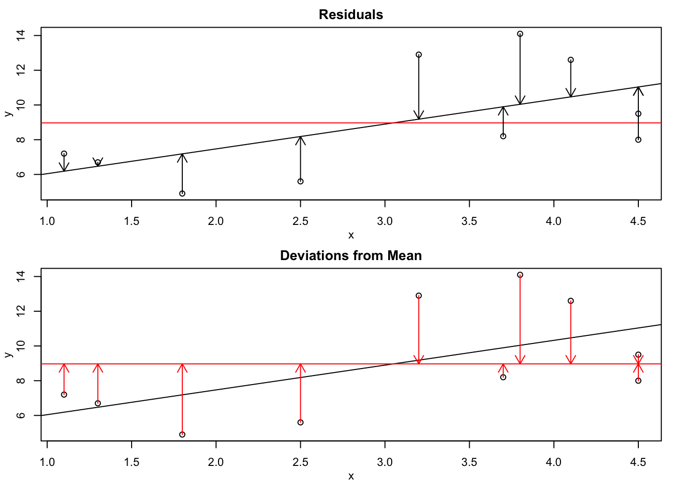
Consult the upper plot in Figure 14.4.1. This is a scatter plot of the data, together with the regression line in black and the line of the average in red. A vertical arrow extends from each data point to the regression line. The point where each arrow hits the regression line is associated with the estimated value of the expectation for that point. The residual is the difference between the value of the response at the origin of the arrow and the value of the response at the tip of its head. Notice that there are as many residuals as there are observations.
The function “
residuals” computes the residuals. The input to the function is the fitted regression model and the output is the sequence of residuals. When we apply the function to the object “fit”, which contains the fitted regression model for the fish data, we get the residuals:
residuals(fit)
##          1          2          3          4          5          6
## -1.5397075 -1.6977999 -2.2857694  0.2279229  3.7158923  4.0594616
##          7          8          9         10
## -2.5849385 -3.0397075  2.1312463  1.0133998
Indeed, 10 residuals are produced, one for each observation. In particular, the residual for the first observation is -1.5397075, which is essentially the value that we obtained.
2
The discrepancy between the value that we computed and the value computed by the function results from rounding up errors. We used the vales of the coefficients that appear in the report. These values are rounded up. The function
residuals uses the coefficients without rounding.
Return to the report produced by the application of the function “
summary” to the fitted regression model. The first component in the report is the formula that identifies the response and the explanatory variable. The second component, the component that comes under the title “Residuals:”, gives a summary of the distribution of the residuals. This summary includes the smallest and the largest values in the sequence of residuals, as well as the first and third quartiles and the median. The average is not reported since the average of the residuals from the regression line is always equal to 0.
The table that contains information on the coefficients was discussed in the previous section. Let us consider the last 3 lines of the report.
The first of the three lines contains the estimated value of the standard deviation of the response from the regression model. If the expectations of the measurements of the response are located on the regression line then the variability of the response corresponds to the variability about this line. The resulting variance is estimated by the sum of squares of the residuals from the regression line, divided by the number of observations minus 2. A division by the number of observation minus 2 produces an unbiased estimator of the variance of the response about the regression model. Taking the square root of the estimated variance produces an estimate of the standard deviation:
sqrt(sum(residuals(fit)^2)/8)
## [1] 2.790787
The last computation is a manual computation of the estimated standard deviation. It involves squaring the residuals and summing the squares. This sum is divided by the number of observations minus 2 (\(10-2=8\)). Taking the square root produces estimate. The value that we get for the estimated standard deviation is 2.790787, which coincides with the value that appears in the first of the last 3 lines of the report.
The second of these lines reports the R-squared of the linear fit. In order to explain the meaning of R-squared let us consider Figure 14.4.1 once again. The two plots in the figure present the scatter plot of the data together with the regression line and the line of the average. Vertical black arrows that represent the residuals from the regression are added to the upper plot. The lower plot contains vertical red arrows that extend from the data points to the line of the average. These arrows represent the deviations of the response from the average.
Consider two forms of variation. One form is the variation of the response from its average value. This variation is summarized by the sample variance, the sum of the squared lengths of the red arrows divided by the number of observations minus 1. The other form of variation is the variation of the response from the fitted regression line. This variation is summarized by the sample variation of the residuals, the sum of squared lengths of the black arrows divided by the number of observations minus 1. The ratio between these two quantities gives the relative variability of the response that remains after fitting the regression line to the data.
The line of the average is a straight line. The deviations of the observations from this straight line can be thought of as residuals from that line. The variability of these residuals, the sum of squares of the deviations from the average divided by the number of observations minus 1, is equal to the sample variance.
The regression line is the unique straight line that minimizes the variability of its residuals. Consequently, the variability of the residuals from the regression, the sum of squares of the residuals from the regression divided by the number of observations minus 1, is the smallest residual variability produced by any straight line. It follows that the sample variance of the regression residuals is less than the sample variance of the response. Therefore, the ratio between the variance of the residuals and the variance of the response is less than 1.
R-squared is the difference between 1 and the ratio of the variances. Its value is between 0 and 1 and it represents the fraction of the variability of the response that is explained by the regression line. The closer the points are to the regression line the larger the value of R-squared becomes. On the other hand, the less there is a linear trend in the data the closer to 0 is the value of R-squared. In the extreme case of R-squared equal to 1 all the data point are positioned exactly on a single straight line. In the other extreme, a value of 0 for R-squared implies no linear trend in the data.
Let us compute manually the difference between 1 and the ratio between the variance of the residuals and the variance of the response:
1-var(residuals(fit))/var(y)
## [1] 0.3297413
Observe that the computed value of R-squared is the same as the value “Multiple R-squared: 0.3297” that is given in the report.
The report provides another value of R-squared, titled Adjusted R-squared. The difference between the adjusted and unadjusted quantities is that in the former the sample variance of the residuals from the regression is replaced by an unbiased estimate of the variability of the response about the regression line. The sum of squares in the unbiased estimator is divided by the number of observations minus 2. Indeed, when we re-compute the ratio using the unbiased estimate, the sum of squared residuals divided by \(10 - 2 = 8\text{,}\) we get:
1-(sum(residuals(fit)^2)/8)/var(y)
## [1] 0.245959
The value of this adjusted quantity is equal to the value “Adjusted R-squared: 0.246” in the report.
Which value of R-squared to use is a matter of personal taste. In any case, for a larger number of observations the difference between the two values becomes negligible.
The last line in the report produces an overall goodness of fit test for the regression model. In the current application of linear regression this test reduces to a test of the slope being equal to zero, the same test that is reported in the second row of the table of coefficients. The \(F\) statistic is simply the square of the \(t\) value that is given in the second row of the table. The sampling distribution of this statistic under the null hypothesis is the \(F\)-distribution on 1 and \(n-2\) degrees of freedom, which is the sampling distribution of the square of the test statistic for the slope. The computed \(p\)-value, “p-value: 0.08255” is the identical (after rounding up) to the \(p\)-value given in the second line of the table.
3
In more complex applications of linear regression, applications that are not considered in this book, the test in the last line of the report and the tests of coefficients do not coincide.
Return to the R-squared coefficient. This coefficient is a convenient measure of the goodness of fit of the regression model to the data. Let us demonstrate this point with the aid of the “
cars” data. In Subsection 14.3.2 we fitted a regression model to the power of the engine as a response and the size of the engine as an explanatory variable. The fitted model was saved in the object called “fit.power”. A report of this fit, the output of the expression summary(fit.power) was also presented. The null hypothesis of zero slope was clearly rejected. The value of R-squared for this fit was 0.6574. Consequently, about 2/3 of the variability in the power of the engine is explained by the size of the engine.
Consider trying to fit a different regression model for the power of the engine as a response. The variable “
length” describes the length of the car (in inches). How well would the length explain the power of the car? We may examine this question using linear regression:
summary(lm(horsepower ~ length, data=cars))
##
## Call:
## lm(formula = horsepower ~ length, data = cars)
##
## Residuals:
##    Min     1Q Median     3Q    Max
## -53.57 -20.35  -6.69  14.45 180.72
##
## Coefficients:
##              Estimate Std. Error t value Pr(>|t|)
## (Intercept) -205.3971    32.8185  -6.259  2.3e-09 ***
## length         1.7796     0.1881   9.459  < 2e-16 ***
## ---
## Signif. codes:  0 '***' 0.001 '**' 0.01 '*' 0.05 '.' 0.1 ' ' 1
##
## Residual standard error: 33.12 on 201 degrees of freedom
##   (2 observations deleted due to missingness)
## Multiple R-squared:  0.308,  Adjusted R-squared:  0.3046
## F-statistic: 89.47 on 1 and 201 DF,  p-value: < 2.2e-16
We used one expression to fit the regression model to the data and to summarize the outcome of the fit.
A scatter plot of the two variables together with the regression line may be produced using the code:
plot(horsepower ~ length, data=cars)
abline(lm(horsepower ~ length, data=cars))
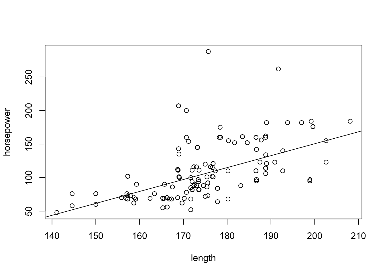
From the examination of the figure we may see that indeed there is a linear trend in the relation between the length and the power of the car. Longer cars tend to have more power. Testing the null hypothesis that the slope is equal to zero produces a very small \(p\)-value and leads to the rejection of the null hypothesis.
The length of the car and the size of the engine are both statistically significant in their relation to the response. However, which of the two explanatory variables produces a better fit?
An answer to this question may be provided by the examination of values of R-squared, the ratio of the variance of the response explained by each of the explanatory variable. The R-squared for the size of the engine as an explanatory variable is 0.6574, which is approximately equal to 2/3. The value of R-squared for the length of the car as an explanatory variable is 0.2933, less than 1/3. It follows that the size of the engine explains twice as much of the variability of the power of the engine than the size of car and is a better explanatory variable.

