Introduction to Statistical Thinking

In this chapter we deal with a Bernoulli response. Such a response has two levels, TRUE or FALSE

¹

The levels are frequently coded as 1 or 0, “success” or “failure”, or any other pair of levels.

, and may emerge as the indicator of an event. Else, it may be associated with a factor with two levels and correspond to the indication of one of the two levels. Such response was considered in Chapter 11 and Chapter 12 where confidence intervals and tests for the probability of an event where discussed in the context of a single sample. In this chapter we discuss the investigation of relations between a response of this form and an explanatory variable.

We start with the case where the explanatory variable is a factor that has two levels. These levels correspond to two sub-populations (or two settings). The aim of the analysis is to compare between the two sub-populations (or between the two settings) the probability of the event.

The discussion in this section is parallel to the discussion in Section Section 13.3. That section considered the comparison of the expectation of a numerical response between two sub-populations. We denoted these sub-populations \(a\) and \(b\) with expectations \(\Expec(X_a)\) and \(\Expec(X_b)\text{,}\) respectively. The inference used the average \(\bar X_a\text{,}\) which was based on a sub-sample of size \(n_a\text{,}\) and the average \(\bar X_b\text{,}\) which was based on the other sub-sample of size \(n_b\text{.}\) The sub-samples variances \(S^2_a\) and \(S^2_b\) participated in the inference as well. The application of a test for the equality of the expectations and a confidence interval where produced by the application of the function t.test to the data.

The inference problem, which is considered in this chapter, involves an event. This event is being examined in two different settings that correspond to two different sub-population \(a\) and \(b\text{.}\) Denote the probabilities of the event in each of the sub-populations by \(p_a\) and \(p_b\text{.}\) Our concern is the statistical inference associated with the comparison of these two probabilities to each other.

Natural estimators of the probabilities are \(\hat P_a\) and \(\hat P_b\text{,}\) the sub-samples proportions of occurrence of the event. These estimators are used in order to carry out the inference. Specifically, we consider here the construction of a confidence interval for the difference \(p_a - p_b\) and a test of the hypothesis that the probabilities are equal.

The methods for producing the confidence intervals for the difference and for testing the null hypothesis that the difference is equal to zero are similar in principle to the methods that were described in the section for making parallel inferences regarding the relations between expectations. However, the derivations of the tools that are used in the current situation are not identical to the derivations of the tools that were used there. The main differences between the two cases is the replacement of the sub-sample averages by the sub-sample proportions, a difference in the way the standard deviation of the statistics are estimated, and the application of a continuity correction. We do not discuss in this chapter the theoretical details associated with the derivations. Instead, we demonstrate the application of the inference in an example.

The variable num.of.doors in the data frame cars describes the number of doors a car has. This variable is a factor with two levels, two and four. We treat this variable as a response and investigate its relation to explanatory variables. In this section the explanatory variable is a factor with two levels and in the next section it is a numeric variable. Specifically, in this section we use the factor fuel.type as the explanatory variable. Recall that this variable identified the type of fuel, diesel or gas, that the car uses. The aim of the analysis is to compare the proportion of cars with four doors between cars that run on diesel and cars that run on gas.

Let us first summarize the data in a \(2 \times 2\) frequency table. The function table may be used in order to produce such a table:

cars <- read.csv("_data/cars.csv")
table(cars$fuel.type,cars$num.of.doors)

##         
##          four two
##   diesel   16   3
##   gas      98  86

When the function table is applied to a combination of two factors then the output is a table of joint frequencies. Each entry in the table contains the frequency in the sample of the combination of levels, one from each variable, that is associated with the entry. For example, there are 16 cars in the data set that have the level four for the variable num.of.doors and the level diesel for the variable fuel.type. Likewise, there are 3 cars that are associated with the combination two and diesel. The total number of entries to the table is \(16 + 3 + 98 + 86 = 203\text{,}\) which is the number of cars in the data set, minus the two missing values in the variable num.of.doors.

A graphical representation of the relation between the two factors can be obtained using a mosaic plot. This plot is produced when the input to the function plot is a formula where both the response and the explanatory variables are factors:

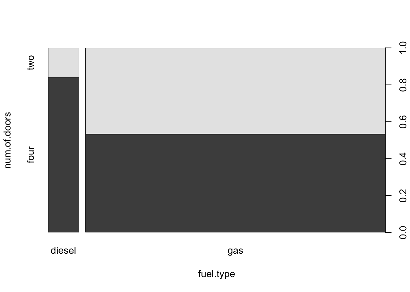
plot(num.of.doors ~ fuel.type,data=cars)

The box plot describes the distribution of the explanatory variable and the distribution of the response for each level of the explanatory variable. In the current example the explanatory variable is the factor fuel that has 2 levels. The two levels of this variable, diesel and gas, are given at the \(x\)-axis. A vertical rectangle is associated with each level. These 2 rectangles split the total area of the square. The total area of the square represents the total relative frequency (which is equal to 1). Consequently, the area of each rectangle represents the relative frequency of the associated level of the explanatory factor.

A rectangle associated with a given level of the explanatory variable is further divided into horizontal sub-rectangles that are associated with the response factor. In the current example each darker rectangle is associated with the level four of the response num.of.door and each brighter rectangle is associated with the level two. The relative area of the horizontal rectangles within each vertical rectangle represent the relative frequency of the levels of the response within each subset associated with the level of the explanatory variable.

Looking at the plot one may appreciate the fact that diesel cars are less frequent than cars that run on gas. The graph also displays the fact that the relative frequency of cars with four doors among diesel cars is larger than the relative frequency of four doors cars among cars that run on gas.

The function prop.test may be used in order test the hypothesis that, at the population level, the probability of the level “four” of the response within the sub-population of diesel cars (the height of the leftmost darker rectangle in the theoretic mosaic plot that is produced for the entire population) is equal to the probability of the same level of the response with in the sub-population of cars that run on gas (the height of the rightmost darker rectangle in that theoretic mosaic plot). Specifically, let us test the hypothesis that the two probabilities of the level “four”, one for diesel cars and one for cars that run on gas, are equal to each other.

The output of the function table may serve as the input to the function prop.test

²

The function prop.test was applied in a previous section in order to test that the probability of an event is equal to a given value (p = 0.5 by default). The input to the function was a pair of numbers: the total number of successes and the sample size. In the current application the input is a \(2 \times 2\) table. When applied to such input the function carries out a test of the equality of the probability of the first column between the rows of the table.

. The Bernoulli response variable should be the second variable in the input to the table whereas the explanatory factor is the first variable in the table. When we apply the test to the data we get the report:

prop.test(table(cars$fuel.type,cars$num.of.doors))

## 
## 	2-sample test for equality of proportions with continuity correction
## 
## data:  table(cars$fuel.type, cars$num.of.doors)
## X-squared = 5.5021, df = 1, p-value = 0.01899
## alternative hypothesis: two.sided
## 95 percent confidence interval:
##  0.1013542 0.5176389
## sample estimates:
##    prop 1    prop 2 
## 0.8421053 0.5326087

The two sample proportions of cars with four doors among diesel and gas cars are presented at the bottom of the report and serve as estimates of the sub-populations probabilities. Indeed, the relative frequency of cars with four doors among diesel cars is equal to \(\hat p_a = 16/(16+3) = 16/19 = 0.8421053\text{.}\) Likewise, the relative frequency of cars with four doors among cars that ran on gas is equal to \(\hat p_b = 98/(98+86) = 98/184 = 0.5326087\text{.}\) The confidence interval for the difference in the probability of a car with four doors between the two sub-populations, \(p_a - p_b\text{,}\) is reported under the title 95 percent confidence interval and is given as \([0.1013542, 0.5176389]\text{.}\)

The null hypothesis, which is the subject of this test, is \(H_0: p_a = p_b\text{.}\) This hypothesis is tested against the two-sided alternative hypothesis \(H_1: p_a \not = p_b\text{.}\) The test itself is based on a test statistic that obtains the value X-squared = 5.5021. This test statistic corresponds essentially to the deviation between the estimated value of the parameter (the difference in sub-sample proportions of the event) and the theoretical value of the parameter (\(p_a - p_b = 0\)). This deviation is divided by the estimated standard deviation and the ratio is squared. The statistic itself is produced via a continuity correction that makes its null distribution closer to the limiting chi-square distribution on one degree of freedom. The \(p\)-value is computed based on this limiting chi-square distribution.

Notice that the computed \(p\)-value is equal to p-value = 0.01899. This value is smaller than 0.05. Consequently, the null hypothesis is rejected at the 5% significance level in favor of the alternative hypothesis. This alternative hypothesis states that the sub-populations probabilities are different from each other.