Introduction to Statistical Thinking

In order to illustrate the statistical inference that compares two expectations let us return to an example that was considered in Chapter 12. The response of interest is the difference in miles-per-gallon between driving in highway conditions and driving in city conditions. This response is produced as the difference between the variable cars$highway.mpg and the variable cars$city.mpg. It is stored in the object dif.mpg, which is a numerical sequence:

cars <- read.csv("_data/cars.csv")
dif.mpg <- cars$highway.mpg - cars$city.mpg

The object heavy was defined in the previous chapter as a sequence with logical components. A component had the value TRUE if the curb weight of the car type associated with this component was above the median level of 2,414 lb. The component obtained the value FALSE if the curb weight did not exceed that level. The logical sequence heavy was used in order to select the subsequences associated with each weight sub-group. Statistical inference was applied separately to each subsequence.

In the current analysis we want to examine directly the relation between the response variable dif.mpg and an explanatory factor variable heavy. In order to do so we redefine the variable heavy to be a factor:

heavy <- factor(cars$curb.weight > 2414)

The variable curb.weight is numeric and the expression cars$curb.weight > 2414 produces a sequence with logical TRUE or FALSE components. This sequence is not a factor. In order to produce a factor we apply the function factor to the sequence. The function factor transforms its input into a factor. Specifically, the application of this function to a sequence with logical components produces a factor with two levels that are given the names TRUE and FALSE

¹

It should be noted that the redefined sequence heavy is no longer a sequence with logical components. It cannot be used, for example, as an index to another sequence in order to select the components that are associated with the TRUE logical value.

.

We want to examine the relation between the response variable dif.mpg and the explanatory factor heavy. Towards that end we produce a plot of the relation with the function plot and test for the equality of the expectations of the response with the function t.test. First the plot:

plot(dif.mpg~heavy)

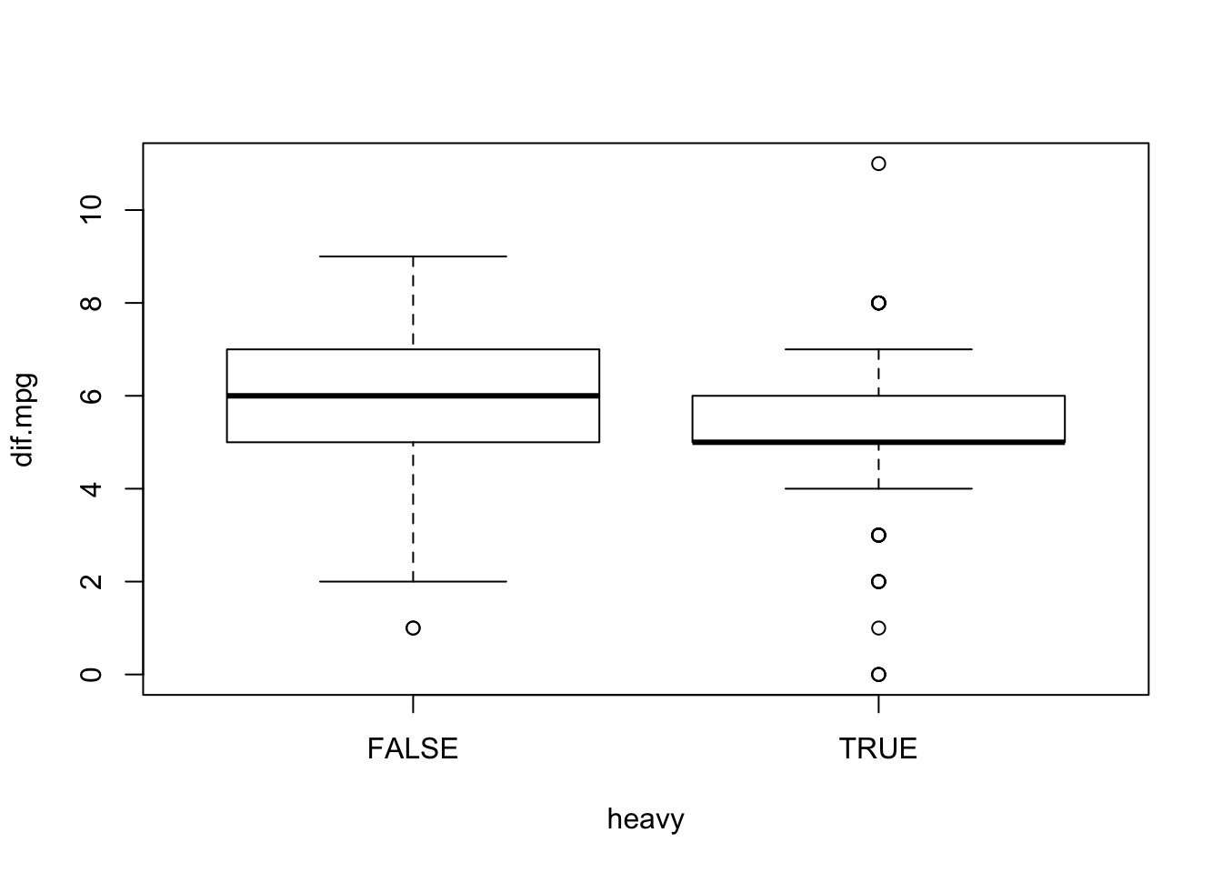
Observe that the figure contains two box plots, one associated with the level FALSE of the explanatory factor and the other with the level TRUE of that factor. The box plots describe the distribution of the response variable for each level of the explanatory factor. Overall, the distribution of the response for heavier cars (cars associated with the level TRUE) tends to obtain smaller values than the distribution of the response for lighter cars (cars associated with the level FALSE).

The input to the function plot is a formula expression of the form: “response\(\;\tilde{}\;\)explanatory.variable”. A formula identifies the role of variables. The variable to the left of the tilde character (\(\;\tilde{}\;\)) in a formula is the response and the variable to the right is the explanatory variable. In the current case the variable dif.mpg is the response and the variable heavy is the explanatory variable.

Let us use a formal test in order to negate the hypothesis that the expectation of the response for the two weight groups is the same. The test is provided by the application of the function t.test to the formula dif.mpg~heavy:

t.test(dif.mpg~heavy)

## 
##  Welch Two Sample t-test
## 
## data:  dif.mpg by heavy
## t = 2.4255, df = 191.56, p-value = 0.01621
## alternative hypothesis: true difference in means is not equal to 0
## 95 percent confidence interval:
##  0.1029150 0.9989315
## sample estimates:
## mean in group FALSE  mean in group TRUE 
##            5.805825            5.254902

The function t.test, when applied to a formula that describes the relation between a numeric response and a explanatory factor with two level, produces a special form of a \(t\)-test that is called the Welch Two Sample \(t\)-test. The statistical model associated with this test assumes the present of two independent sub-samples, each associated with a level of the explanatory variable. The relevant parameters for this model are the two expectations and the two variances associated with the sub-samples.

The hypotheses tested in the context of the Welch test are formulated in terms of the difference between the expectation of the first sub-sample and the expectation of the second sub-sample. In the default application of the test the null hypothesis is that the difference is equal to 0 (or, equivalently, that the expectations are equal to each other). The alternative is that the difference is not equal to 0 (hence, the expectations differ).

The test is conducted with the aid of a test statistic. The computed value of the test statistic in this example is t = 2.4255. Under the null hypothesis the distribution of the test statistic is (approximately) equal to the \(t\)-distribution on df = 191.561 degrees of freedom. The resulting \(p\)-value is p-value = 0.01621. Since the computed \(p\)-value is less than 0.05 we reject the null hypothesis with a significance level of 5% and declare that the expectations are not equal to each other.

The bottom part of the report presents points estimates and a confidence interval. The point estimates of the two expectations are the sub-samples averages. The estimated value of the expected difference in miles-per-gallon for lighter cars is 5.805825, which is the average of the measurements associated with the level FALSE. The estimated value of the expected difference for heavier cars is 5.254902, the average of measurements associated with the level TRUE.

The point estimate for the difference between the two expectations is the difference between the two sample averages: \(5.805825 - 5.254902 = 0.550923\text{.}\) A confidence interval for the difference between the expectations is reported under the title 95 percent confidence interval:. The computed value of the confidence interval is \([0.1029150, 0.9989315]\text{.}\)

In the rest of this section we describe the theory behind the construction of the confidence interval and the statistical test.

Consider the statistical model that is used for the construction of the confidence interval. The main issue is that the model actually deals with two populations rather than one population. In previous theoretical discussions we assumed the presence of a single population and a measurement taken for the members of this population. When the measurement was considered as a random variable it was denoted by a capital Latin letter such as \(X\text{.}\) Of concern were characteristics of the distribution of \(X\) such as \(\Expec(X)\text{,}\) the expectation of \(X\text{,}\) and \(\Var(X)\text{,}\) the variance.

In the current investigation two populations are considered. One population is the sub-population associated with the first level of the factor and the other population is associated with the second level. The measurement is taken for the members of both sub-populations. However, the measurement involves two random variables, one associated with the first sub-population and the other associated with the second sub-population. Moreover, the distribution of the measurement for one population may differ from the distribution for the other population. We denote the random variable associated with the first sub-population by \(X_a\) and the one associated with the other sub-population by \(X_b\text{.}\)

Consider the example in which the measurement is the difference in miles-per-gallon between highway and city driving conditions. In this example \(X_a\) is the measurement for cars with curb weight up to 2,414 lb and \(X_b\) is the same measurement for cars with curb weight above that threshold.

The random variables \(X_a\) and \(X_b\) may have different distributions. Consequently, the characteristics of their distributions may also vary. Denote by \(\Expec(X_a)\) and \(\Expec(X_b)\) the expectations of the first and second random variable, respectively. Likewise, \(\Var(X_a)\) and \(\Var(X_b)\) are the variances of the two random variables. These expectations and variances are subjects of the statistical inference.

The sample itself may also be divided into two sub-samples according to the sub-population each observation originated from. In the example, one sub-sample is associated with the lighter car types and the other sub-sample with the heavier ones. These sub-samples can be used in order to make inference with respect to the parameters of \(X_a\) and \(X_b\text{,}\) respectively. For example, the average of the observations from first sub-sample, \(\bar X_a\text{,}\) can serve as the estimator of the of the expectation \(\Expec(X_a)\) and the second sub-sample’s average \(\bar X_b\) may be used in order to estimate \(\Expec(X_b)\text{.}\)

Our goal in this section is to construct a confidence interval for the difference in expectations \(\Expec(X_a)-\Expec(X_b)\text{.}\) A natural estimator for this difference in expectations is the difference in averages \(\bar X_a- \bar X_b\text{.}\) The average difference will also serve as the basis for the construction of a confidence interval.

Recall that the construction of the confidence interval for a single expectation was based on the sample average \(\bar X\text{.}\) We exploited the fact that the distribution of \(Z = (\bar X - \Expec(X)/\sqrt{\Var(X)/n}\text{,}\) the standardized sample average, is approximately standard Normal. From this Normal approximation we obtained an approximate 0.95 probability for the event

where \(1.96 = \mbox{\texttt{qnorm(0.975)}}\) is the 0.975-percentile of the standard Normal distribution

²

In the case where the sample size is small and the observations are Normally distributed we used the \(t\)-distribution instead. The percentile that was used in that case was qt(0.975,n-1), the 0.975 percentile of the \(t\)-distribution on \(n-1\) degrees of freedom.

. Substituting the estimator \(S\) for the unknown variance of the measurement and rewriting the event in a format that puts the expectation \(\Expec(X)\) in the center, between two boundaries, produced the confidence interval:

Similar considerations can be used in the construction of a confidence interval for the difference between expectations on the basis of the difference between sub-sample averages. The deviation \(\{\bar X_a- \bar X_b\} - \{\Expec(X_a)- \Expec(X_b)\}\) between the difference of the averages and the difference of the expectations that they estimate can be standardized. By the Central Limit Theorem one may obtain that the distribution of the standardized deviation is approximately standard Normal.

Standardization is obtained by dividing by the standard deviation of the estimator. In the current setting the estimator is the difference between the averages. The variance of the difference is given by

where \(n_a\) is the size of the sub-sample that produces the sample average \(\bar X_a\) and \(n_b\) is the size of the sub-sample that produces the sample average \(\bar X_b\text{.}\) Observe that both \(\bar X_a\) and \(\bar X_b\) contribute to the variability of the difference. The total variability is the sum of the two contributions

³

It can be proved mathematically that the variance of a difference (or a sum) of two independent random variables is the sum of the variances. The situation is different when the two random variables are correlated.

. Finally, we use the fact that the variance of the sample average is equal to he variance of a single measurement divided by the sample size. This fact is used for both averages in order to obtain a representation of the variance of the estimator in terms of the variances of the measurement in the two sub-population and the sizes of the two sub-samples.

The standardized deviation takes the form:

When both sample sizes \(n_a\) and \(n_b\) are large then the distribution of \(Z\) is approximately standard Normal. As a corollary from the Normal approximation one gets that \(\Prob(-1.96 \leq Z \leq 1.96) \approx 0.95\text{.}\)

The values of variances \(\Var(X_a)\) and \(\Var(X_b)\) that appear in the definition of \(Z\) are unknown. However, these values can be estimated using the sub-samples variances \(S_a^2\) and \(S_b^2\text{.}\) When the size of both sub-samples is large then these estimators will produce good approximations of the unknown variances:

The event \(\{-1.96 \leq Z \leq 1.96\}\) may be approximated by the event:

The approximation results from the use of the sub-sample variances as a substitute for the unknown variances of the measurement in the two sub-populations. When the two sample sizes \(n_a\) and \(n_b\) are large then the probability of the given event will also be approximately equal to 0.95.

Finally, reexpressing the least event in a format that puts the parameter \(\Expec(X_a)- \Expec(X_b)\) in the center will produce the confidence interval with boundaries of the form:

In order to illustrate the computations that are involved in the construction of a confidence interval for the difference between two expectations let us return to the example of difference in miles-per-gallon for lighter and for heavier cars. Compute the two sample sizes, sample averages, and sample variances:

table(heavy)
tapply(dif.mpg,heavy,mean)
tapply(dif.mpg,heavy,var)

## heavy
## FALSE  TRUE 
##   103   102

##    FALSE     TRUE 
## 5.805825 5.254902

##    FALSE     TRUE 
## 2.020750 3.261114

Observe that there 103 lighter cars and 102 heavier ones. These counts were obtained by the application of the function table to the factor heavy. The lighter cars are associated with the level FALSE and heavier cars are associated with the level TRUE.

The average difference in miles-per-gallon for lighter cars is 5.805825 and the variance is 2.020750. The average difference in miles-per-gallon for heavier cars is 5.254902 and the variance is 3.261114. These quantities were obtained by the application of the functions mean or var to the values of the variable dif.mpg that are associated with each level of the factor heavy. The application was carried out using the function tapply.

The computed values of the means are equal to the vales reported in the output of the application of the function t.test to the formula dif.mpg~heavy. The difference between the averages is \(\bar x_a - \bar x_b = 5.805825 - 5.254902 = 0.550923\text{.}\) This value is the center of the confidence interval. The estimate of the standard deviation of the difference in averages is:

Therefore, the confidence interval for the difference in expectations is

which is (essentially) the confidence interval that is presented in the report

⁴

The confidence interval given in the output of the function t.test is \([0.1029150, 0.9989315]\text{,}\) which is very similar, but not identical, to the confidence interval that we computed. The discrepancy stems from the selection of the percentile. We used the percentile of the normal distribution 1.96 = qnorm(0.975). The function t.test, on the other hand, uses the percentile of the \(t\)-distribution 1.972425 = qt(0.975,191.561). Using this value instead would give \(0.550923 \pm 1.972425 \cdot 0.227135\text{,}\) which coincides with the interval reported by t.test. For practical applications the difference between the two confidence intervals are not negligible.

.

The statistical model that involves two sub-populations may be considered also in the context of hypothesis testing. Hypotheses can be formulated regarding the relations between the parameters of the model. These hypotheses can be tested using the data. For example, in the current application of the \(t\)-test, the null hypothesis is \(H_0: \Expec(X_a) = \Expec(X_b)\) and the alternative hypothesis is \(H_1: \Expec(X_a) \not= \Expec(X_b)\text{.}\) In this subsection we explain the theory behind this test.

Recall that the construction of a statistical test included the definition of a test statistic and the determination of a rejection region. The null hypothesis is rejected if, and only if, the test statistic obtains a value in the rejection region. The determination of the rejection region is based on the sampling distribution of the test statistic under the null hypothesis. The significance level of the test is the probability of rejecting the null hypothesis (i.e., the probability that the test statistic obtains a value in the rejection region) when the null hypothesis is correct (the distribution of the test statistic is the distribution under the null hypothesis). The significance level of the test is set at a given value, say 5%, thereby restricting the size of the rejection region.

In the previous chapter we consider the case where there is one population. For review, consider testing the hypothesis that the expectation of the measurement is equal to zero (\(H_0: \Expec(X) = 0\)) against the alternative hypothesis that it is not (\(H_1: \Expec(X) \not = 0\)). A sample of size \(n\) is obtained from this population. Based on the sample one may compute a test statistic:

where \(\bar X\) is the sample average and \(S\) is the sample standard deviation. The rejection region of this test is \(\{|T| > \mbox{\texttt{qt(0.975,n-1)}}\}\text{,}\) for qt(0.975,n-1) the 0.975-percentile of the \(t\)-distribution on \(n-1\) degrees of freedom.

Alternatively, one may compute the \(p\)-value and reject the null hypothesis if the \(p\)-value is less than 0.05. The \(p\)-value in this case is equal to \(\Prob(|T| > |t|)\text{,}\) where \(t\) is the computed value of the test statistic. The distribution of \(T\) is the \(t\)-distribution of \(n-1\) degrees of freedom.

A similar approach can be used in the situation where two sub-population are involved and one wants to test the null hypothesis that the expectations are equal versus the alternative hypothesis that they are not. The null hypothesis can be written in the form \(H_0:\Expec(X_a) - \Expec(X_b) = 0\) with the alternative hypothesis given as \(H_1:\Expec(X_a) - \Expec(X_b) \not = 0\text{.}\)

It is natural to base the test static on the difference between sub-samples averages \(\bar X_a - \bar X_b\text{.}\) The \(T\) statistic is the ratio between the deviation of the estimator from the null value of the parameter, divided by the (estimated) standard deviation of the estimator. In the current setting the estimator is difference in sub-samples averages \(\bar X_a - \bar X_b\text{,}\) the null value of the parameter, the difference between the expectations, is 0, and the (estimated) standard deviation of the estimator is \(\sqrt{S_a^2/n_a + S_b^2/n_b}\text{.}\) It turns out that the test statistic in the current setting is:

Consider as a measurement the difference in miles-per-gallon. Define the sub-population \(a\) to the lighter cars and the sub-population \(b\) to be the heavier cars. Recall that the sub-sample sizes are \(n_a =103\) and \(n_b=102\text{.}\) Also, the sub-sample averages are \(\bar x_a = 5.805825\) and \(\bar x_b =5.254902\text{,}\) and the sub-sample variances are \(s^2_a = 2.020750\) and \(s_b^2 = 3.261114\text{.}\)

In order to calculate the observed value of the test statistic we use once more the fact that the difference between the averages is \(\bar x_a - \bar x_b = 5.805825 - 5.254902 = 0.550923\) and the estimated value of the standard deviation of the sub-samples average difference is:

It follows that the observed value of the \(T\) statistic is

which, after rounding up, is equal to the value presented in the report that was produced by the function t.test.

The \(p\)-value is computed as the probability of obtaining values of the test statistic more extreme than the value that was obtained in our data. The computation is carried out under the assumptions of the null hypothesis. The limit distribution of the \(T\) statistic, when both sub-sample sizes \(n_a\) and \(n_b\) are large, is standard Normal. In the case when the measurements are Normally distributed then a refined approximation of the distribution of the statistic is the \(t\)-distribution. Both the standard Normal and the \(t\)-distribution are symmetric about the origin.

The probability of obtaining a value in either tails for a symmetric distribution is equal to twice the probability of obtaining a value in the upper tail:

The function t.test computes the \(p\)-value using the \(t\)-distribution. For the current data, the number of degrees of freedom that are used in this approximation

⁵

The Weltch \(t\)-test for the comparison of two means uses the \(t\)-distribution as an approximation of the null distribution of the \(T\) test statistic. The number of degrees of freedom is computed by the formula: \(\mbox{\texttt{df}} = (v_a + v_b)^2/\{v_a^2/(n_a-1) + v_b^2/(n_b-1)\}\text{,}\) where \(v_a = s_a^2/n_a\) and \(v_b = s_b^2/n_b\text{.}\)

is df = 191.561. When we apply the function pt for the computation of the cumulative probability of the \(t\)-distribution we get:

2*(1-pt(2.4255,191.561))

## [1] 0.01621458

which (after rounding) is equal to the reported \(p\)-value of 0.01621. This \(p\)-value is less than 0.05, hence the null hypothesis is rejected in favor of the alternative hypothesis that assumes an effect of the weight on the expectation.