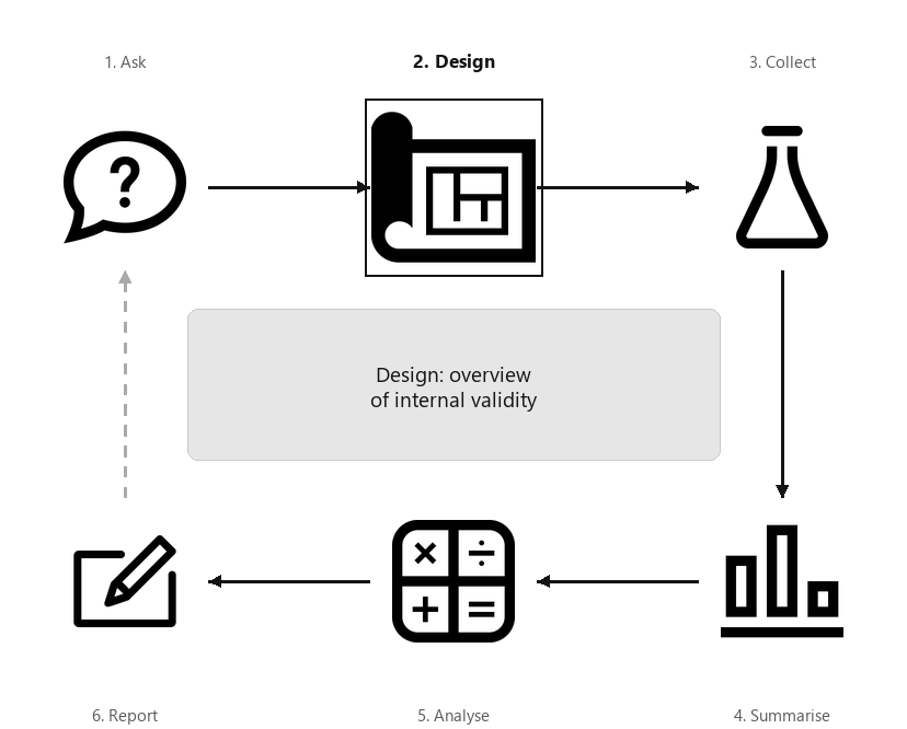
A diagram showing the six steps of research, arranged in a cycle: Ask, Design, Collect, Classify and summarise, Analyse, Report. Step 2 (Design) is highlighted, captioned “Design: overview of internal validity”.
Section3.1Introduction: internal and external validity
An RQ asks about a population. However, studying every member of a population is generally impossible due to cost, time, ethics, logistics and/or practicality. A subset of the population (a sample) is studied, comprising some individuals from the population. Countless different samples are possible.
Being able to generalise about the population of interest from studying a sample is called external validity. Chapter 6 discusses how to select a suitable sample to study to enhance external validity.
Apart from being externally valid, well-designed research studies should be internally valid. An internally valid study allows the researchers to focus on the relationship of interest between the response and explanatory variables, by eliminating, or accounting for, other sources of variation in the values of the response variable. These other sources are discussed in the rest of this chapter.
A study with high internal validity shows that the changes in the response variable can be (at least partially) attributed to changes in the explanatory variables; other explanations have been ruled out.
One challenge of research is learning about the relationship between the response and explanatory variables, when the value of the response variable can also be influenced by other factors.
Studies with low internal validity leave open other possibilities, apart from changes in the value of the explanatory variable, to explain changes in the value of the response variable. Ideally, all studies should be designed to be internally valid as far as possible. Internal validity is studied in more detail in Chapter 7. Different research studies (Chapter 4) differ in the extent to which they can achieve internal validity.
For students in a large university course, is the average typing speed (in words per minute) the same for those aged under \(25\) (“younger”) and \(25\) or over (“older”)?
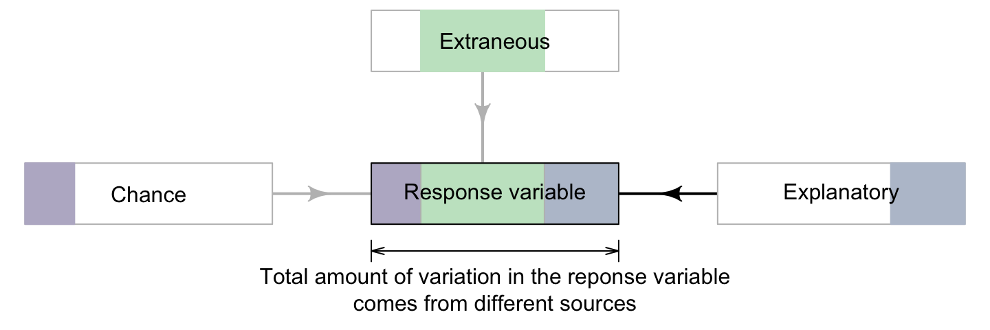
The typing speed (the response variable) of the many individuals will vary: every student in the study recording exactly the same typing speed is highly unlikely. The variation in the values of students’ typing speeds (Figure 3.7) may be due to:
the explanatory variable (Section 3.3). The values of the explanatory variable may influence the values of the response variable. Of course, they may not either; the purpose of the study is to find if, or to what extent, this is true. In this example, the explanatory variable is the age group of the student, which may impact typing speed.
other variables, called extraneous variables (Section 3.4). Other variables (apart from the explanatory variable) may influence the response variable (perhaps more than the explanatory variable), such as “sex of the person”, or “whether the person wears glasses”. The impact of these variables can be accommodated if the study is designed appropriately.
chance (or randomness, or natural variation) (Section 3.5). The same person doing the same thing repeatedly under the same conditions will not record exactly the same typing speed every attempt. This is unavoidable, but good research design can minimise the size of this variation.
Designing studies to maximise internal validity requires identifying important extraneous variables, and eliminating (as far as possible) anything that obscures the relationship between the response and explanatory variables.
In the typing-speed study, suppose younger students were always asked to use their dominant hand, and older students always asked to use their non-dominant hand. Younger students would probably have a faster average typing speed, simply because they use their dominant hands (not due to age). This research design would produce a study with poor internal validity.
Internal validity is one of the most important properties of scientific studies, and is relevant for reasoning about evidence more generally. Designing studies to maximise internal validity is the focus of Chapter 7.
Data collection is often tedious, time-consuming and expensive: you usually get one chance to collect data. In contrast, data (once collected) can be analysed as many times as necessary. Design the study properly the first time!
Section3.3Variation due to changes in the explanatory variable
Changes in the values of the explanatory variable may, or may not, be associated with changes in the values of the response variable. If nothing else influenced the values of the response variable, life would be easy: any change of a given size in the value of the explanatory variable would always result in a change of the same size in the value of the response variable.
In the typing-speed study (Example 3.5), the explanatory variable is the age group. If nothing else influenced typing speed, every younger student would record the same typing speed every time, and every older student would record the same typing speed every time. This is clearly unreasonable.
Section3.4Variation due to changes in the extraneous variables
Other variables (besides the explanatory variable) almost certainly exist which are associated with changes in the value of the response variable. These are called extraneous variables.
In the typing-speed study (Example 3.5), potential extraneous variables may include age, the presence or absence of certain medical conditions, the level of familiarity with computers, whether the person wears glasses, etc.
The impact of some extraneous variables on the response variable can be reduced by fixing the values of the variable. These variables are called control variables.
In the typing-speed study (Example 3.5), typing speeds would vary greatly if students used different types of keyboards; for example, if some students used mechanical keyboards, and some used on-screen keyboards (e.g., on a tablet). The impact of age is easier to detect if all students use the same keyboards, as this would reduce the variation in the typing speeds.
If many other variables are fixed in value (i.e., are control variables), the relationship between the explanatory and response variables is far easier to detect and measure. However, using too many control variables may limit the population, and hence the generalisability of the results. In the typing-speed study, for example, restricting the study to left-handed males who do not wear glasses would restrict the results to a very narrow group of people.
All extraneous variables are, by definition, related to the response variable. They may or may not also be associated with the explanatory variable. Extraneous variables also related to the explanatory variable are called confounding variables (or confounders); see Figure 3.21 (left panel). A confounding variable can obscure the true relationship between the response and explanatory variables.
Confounding variables are associated with both the response and explanatory variables. This does not necessarily mean the value of the confounding variable causes changes in the values of the response or explanatory variables.
Example3.18.Confounding variables and associations.
Consider a study comparing the proportion of females and males wearing sunglasses while walking in a local park. To determine if the variable “whether it is raining” is an extraneous variable, we ask:
We do not ask if the presence of rain changes the sex of the person; we ask if the presence of rain is associated with different proportions of males and females walking in the presence of rain. It may be the case (for example) that males are more likely to walk in the rain than females, so “whether it is raining” may be a confounding variable (but it is not obvious).
A relationship between the response and explanatory variables may be apparent, but only because both of these variables are associated with the confounding variable (Figure 3.21). No relationship actually exists between the response and explanatory variables.
People who carry cigarette lighters are more likely to get lung cancer. The reason this relationship exists, however, is because of a confounding variable. “Whether the person is a smoker” is probably associated with both the response and explanatory variables:
Among university students, is the percentage of females who know their own blood pressure the same as the percentage of males who know their own blood pressure?
For this RQ, the explanatory variable is the sex of person, and the response variable is whether a student knows their own blood pressure. A potential confounding variable is “The program of study”, since this is (potentially) related to both the response and explanatory variables:
“Program of study” is related to sex (the explanatory variable): a higher percentage of females study nursing, while a greater percentage of males study engineering (at least, in Australia).
“Program of study” is related to knowing your blood pressure (the response variable): nursing students probably practice taking each other’s blood pressures so probably know their own, whereas engineering students do not.
Managing confounding is very important, as ignoring confounding can completely change the observed relationship between the response and explanatory variables (see Section 15.7) and hence can compromise internal validity. Managing confounding is discussed in Section 7.2.
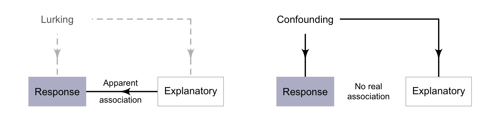
Two diagrams side by side showing confounding. Left: the confounding variable is unmeasured (lurking) and creates an apparent association. Right: in extreme confounding, no real association exists between the response and explanatory variables.
Figure3.21.Confounding variables are extraneous variables associated with the response and explanatory variables. Left: If the confounding variable is not measured (and so a lurking variable is present), an apparent association exists between the response and explanatory variables. Usually, confounding is not as extreme as shown in this diagram, and the confounding variable may slightly change the relationship between response and explanatory variables. Right: In extreme confounding situations, as shown here, no real association exists between the response and explanatory variables; the association is explained by a confounding variable.
If the values of potential confounding variables are recorded, their impact can be managed. However, sometimes the values of the confounding variables are not recorded (perhaps due to poor design); then, they are called lurking variables (Figure 3.21, left panel). Lurking variables can lead to wrong conclusions.
A lurking variable is an extraneous variable associated with the response and explanatory variables (that is, is a confounding variable), but whose values are not recorded in the study data.
Hot plastic was introduced in the mold, pressed for \(10\secs\text{,}\) and removed. Another batch was then introduced into the same mold, pressed for \(20\secs\text{,}\) and so on, the time increasing with each batch.
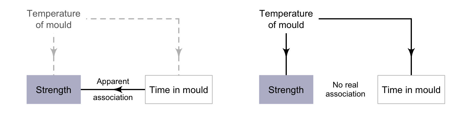
Greater time in the mould (explanatory variable) was found to be associated with greater plastic strength (response variable). However, mould temperature was later found to be a lurking variable, since it was associated with both the response and explanatory variables:
higher mould temperatures (the lurking variable) were experienced by later batches with longer mould times (the explanatory variable), since the mould was hotter for the later batches.
Two diagrams side by side. Left: mould time appears to influence plastic strength. Right: mould temperature is the true cause, as a lurking variable influencing both time in mould and strength.
Figure3.24.An example of a lurking variable. Left: the relationship as originally understood. Right: the relationship after the lurking variable was eventually exposed.
extraneous variables are, by definition, always associated with the response variable. If they are not recorded, and so the researchers are unaware of them, they become part of unexplained chance.
Table3.25.The relationships between extraneous, confounding and lurking variables. Entries in italics indicate different types of extraneous variables.
To avoid lurking variables, researchers generally collect lots of information that may be relevant about the individuals in the study (such as age and sex if the study involves people) and circumstances of the individuals in the study (such as the temperature at the time of data collection), in case they are confounding variables.
[58] reviewed numerous studies that used double-fortified salt to manage iodine and iron deficiencies. They concluded that the internal validity of studies was “generally weak” (p. 265) due, in part, to “unaccounted confounders” (i.e., lurking variables).
Section3.5Variation due to natural variation (chance)
Chance variation (or natural variation) refers to variation that cannot otherwise be explained: even repeating a study exactly the same way every time on the same individuals will not always produce the same values of the response variable.
The influence of the explanatory variable is hard to detect if the amount of chance variation contributing to the response variable overwhelms the amount of variation produced by changes in the value of the explanatory variable. Minimising the amount of the chance variation requires using good design principles, and measuring as many other extraneous variables that may explain variation in the response variable as reasonable.
taking \(30\) observations from one younger student would tell us about variation in that student’s typing speed, but very little about variation in younger students’ typing speeds more generally.
taking one observation from \(30\) different younger students would tell us about variation in younger students’ typing speeds in general. We only have one measurement from each student, but since we might expect that the same person to produce similar (not identical) typing speeds, this should not be a big problem.
taking three observations from each of \(10\) different younger students would tell us about variation in younger students’ typing speeds in general, and a little about the variation in each students’ typing speeds too.
Research questions are about populations, but samples are studied in practice. Studies that use a sample that represents the population of interest are called externally valid.
In a research study, the main interest is usually the relationship between a response variable and explanatory variable. Well-designed studies that allow the researchers to focus on this relationship have good internal validity. Such studies eliminate, or account for, other explanations for the variation in the values of the response variable.
The values of the response variable can be influenced by more than just the explanatory variable, such as extraneous variables (other variables not of primary interest), and chance.
Some extraneous variables are also related to the explanatory variable, and are called confounding variables (and are lurking variables if not recorded). If the research design makes it difficult to separate the relationship between the response and explanatory variable from other possible causes, the study has poor internal validity.
They recorded the age, height, weight, and resting metabolic rate of all subjects who completed the \(4.5\kms\) ride. Each subject was allocated to ride both with and without cargo.
The Giant Mine in Yellowknife, Canada, ceased operation in 1999 after \(50\) years, during which \(237\,000\) tonnes of arsenic trioxide was released. [51] examined the arsenic concentration in \(25\) lakes within a \(25\kms\) radius of the mine \(11\) years after the mine closed, to determine if the arsenic concentration was related to the distance of the lake from the mine. They also recorded:
A study examined the relationship between diet quality and depression in Australian adolescents [53]. The researchers used a sample of \(7\,114\) adolescents aged \(10\)--\(14\) years old, and also measured information about (p. 435):
... age, gender, socioeconomic status, parental education, parental work status, family conflict, poor family management, dieting behaviours, body mass index, physical activity, and smoking...
A newspaper article [18] reported that “Women who drank green tea at least three times a week were \(14\) per cent less likely to develop a cancer of the digestive system”. However, the final paragraph of the article notes that:
A study recorded the lung capacity (using Forced Expiratory Volume, or FEV, in litres) of children aged \(3\) to \(19\) [[26]; [1]], and also recorded whether or not the children were smokers. One finding was that children who smoke have a larger average FEV (i.e., larger average lung capacity) than children who do not smoke, in general.
Consider a study to determine if the percentage of children who consume Ready-To-Eat-Cereals (RTEC) for breakfast is the same for children aged between \(5\) and \(10\text{,}\) as for children aged between \(11\) and \(15\text{.}\) The researchers also measured the age of the child, the number of siblings living with the child, and the sex of the child.
Which of these variables are extraneous variables? The sex of the child; whether the child consumes RTEC; the age group of the child; the age of the child; the number of siblings living with the child.
Extraneous variables are variables that are related to the response variable. Which of the following types of variables are special types of extraneous variables?
A study of New Zealanders found that people wearing hearing aids were more likely to have grey hair than people not wearing hearing aids. What confounding variable is likely to be present?
Researchers are studying a new (but expensive) insecticide that is claimed to be more effective for use in apple orchards than other (cheaper) insecticides. A study found that apple orchards where the farmers chose to use the new insecticide had a similar number of insects per tree than orchards where the farmers chose not to use the new insecticide. What confounding variable is likely to be present?
An agricultural study recorded the wheat yield for \(18\) organic farms and \(29\) conventional farms. Farms across North Dakota and Kansas (USA) were used for the study, and the yield (in tonnes per hectare) was recorded from each farm. The organic farms were generally smaller than the non-organic farms, and located in areas with better soil quality.
A study of school teachers found a relationship between the average number of children plus grandchildren for the teacher, and having high blood pressure.