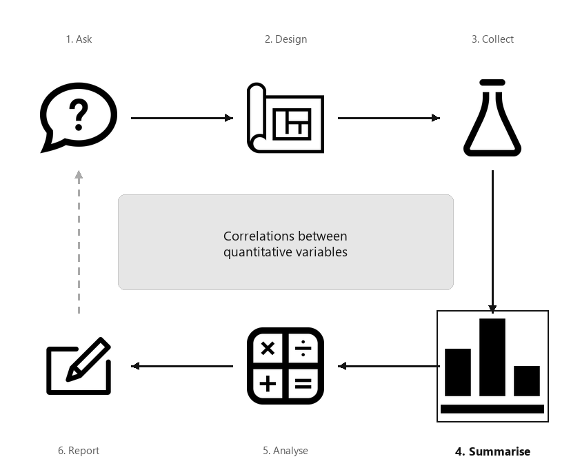
A diagram showing the six steps of research, arranged in a cycle: Ask, Design, Collect, Classify and summarise, Analyse, Report. Step 4 (Summarise) is highlighted, captioned “Correlations between quantitative variables”.
Correlational RQs ask about the relationship between two quantitative variables. Scatterplots are useful for this purpose, and the relationship is usually described numerically using a correlation coefficient or \(R^2\text{.}\)
Scatterplots display the relationship between two quantitative variables. Conventionally, and when appropriate, the response variable (denoted \(y\)) is shown on the vertical axis, and the explanatory variable (denoted \(x\)) is shown on the horizontal axis. Two quantitative variables are measured on each individual, and a point is placed on the scatterplot for each individual (unit of analysis) to indicate the values of the two variables. In some cases, which variable is denoted \(x\) and which is \(y\) is not important (e.g., see Exercise Exercise 33.9.15.)
As with any graph, describing the message in the graph is important, because the purpose of a graph is to display the information in the clearest, simplest possible way.
[144] examined the relationship between the age of \(n = 78\) male red deer and the weight of their molars. The data (Table Table 16.2) comprises two quantitative variables, and both measurements are made on the same individuals (i.e., male red deer).
The scatterplot (Fig. Figure 16.3) shows one dot for each deer (individual). The response variable is the molar weight, which is on the vertical axis and denoted \(y\text{.}\) The explanatory variable is the deer age, which is on the horizontal axis and denoted \(x\text{.}\)
For instance, one deer is just over \(4\) years of age (so \(x\) has a value a bit larger than \(4\)), and has a molar weight of \(2.42\) g (so that \(y = 2.42\)). This is the first deer listed in Table Table 16.2.
The purpose of a graph is to facilitate understanding of the data. For a scatterplot, the form, direction, and variation in the relationship (or the strength of the relationship) are described.
Variation: the amount of variation in the relationship. A small amount of variation in the response variable for given values of the explanatory variable means the relationship is strong; a lot of variation in the response variable for given values of the explanatory variable means the relationship is weak. Describing the variation can be difficult; an objective, numerical way to do so is explained in Sect. Section 16.4.
Anything unusual or noteworthy should also be discussed. These features explain the type of relationship (form; direction), and the strength of that relationship (variation). Examples are shown in Fig. Figure 16.5.
For the red-deer data (Fig. Figure 16.3), the relationship is approximately linear (form) with a negative direction (older deer generally have lighter teeth); the variation is, perhaps, moderate.
[26] (cited by [1]) measured the lung capacity of children in Boston (using forced expiratory volume, FEV, in litres). The scatterplot (Fig. Figure 16.8) is curved (form), where older children have larger FEVs, in general (direction). The variation in FEV gets larger for taller youth.
Scatterplot of FEV vs height for children in Boston, showing three panels: the raw scatterplot, an inappropriate linear fit, and the appropriate non-linear fit with increasing variation.
Section16.4Numerical summary: correlation coefficient and R^2
Subsection16.4.1Correlation coefficients
In general, summarising the relationship between two quantitative variables is difficult, because the possible relationships vary greatly (consider the variety in the scatterplots shown in Fig. Figure 16.5).
However, if we focus only on approximately linear relationships, the best way to numerically summarise the relationship between the variables is to use a correlation coefficient. Both quantitative variables can also be numerically summarised individually.
The Pearson correlation coefficient measures the strength and direction of the linear relationship between two quantitative variables. Its value is always between \(-1\) and \(+1\text{.}\)
Only the Pearson correlation coefficient is discussed in this book (and usually referred to as the ’correlation coefficient’), but other correlation coefficients also exist (such as the Spearman or Kendall correlation coefficients), which may be used for increasing-only or decreasing-only non-linear relationships).
In the population, the unknown value of the correlation coefficient is denoted \(\rho\) (’rho’); in the sample, the value of the correlation coefficient is denoted \(r\text{.}\) As usual, \(r\) (the statistic) is an estimate of \(\rho\) (the parameter), and the value of \(r\) is likely to be different in every sample (that is, sampling variation exists).
The values of \(\rho\) and \(r\) are always between \(-1\) and \(+1\text{.}\) The sign indicates whether the relationship has a positive or negative linear association, and the value of the correlation coefficient describes the strength of the relationship, as follows.
\(r = -1\) indicates a perfect, negative relationship. By ’perfect’, we mean that each value of \(x\) always produces the same value of \(y\text{;}\) the negative value means larger values of \(y\) are associated with smaller values of \(x\text{.}\)
values of \(r\) between \(-1\) and \(0\) indicates a negative relationship. Each value of \(x\) produces a range of values of \(y\text{,}\) and larger values of \(y\) are associated with smaller values of \(x\) (in general).
\(r = 0\) indicates no linear relationship between the variables: knowing how the value of \(x\) changes tells us nothing about how the corresponding value of \(y\) changes. The best prediction of \(y\) for any value of \(x\) would be the mean of \(y\text{;}\) i.e., the value of \(\bar{y}\text{.}\)
values of \(r\) between \(0\) and \(+1\) indicates a positive relationship. Each value of \(x\) produces a range of values of \(y\text{,}\) and larger values of \(y\) are associated with larger values of \(x\) (in general).
\(r = +1\) indicates a perfect, positive relationship. By ’perfect’, we mean that each value of \(x\) always produces the same value of \(y\text{;}\) the positive value means larger values of \(y\) are associated with larger values of \(x\text{.}\)
Almost all values of \(r\) seen in practice are between the extremes of \(r = -1\) and \(r = +1\text{.}\) Guessing the values of the correlation coefficient from a scatterplot is very difficult.
Numerous example scatterplots were shown in Sect. Section 16.3 (Fig. Figure 16.5). A correlation coefficient is not relevant for Plots C, D or E, as those relationships are not linear. For the others:
[145] and [146] explored the relationship between water temperature and fertilisation rates for sand dollars (Fig. Figure 16.14). The correlation coefficient is \(r = -0.71\) (left panel), which might suggest that higher temperatures result in lower fertilisation rates. However, a curved relationship is apparent (right panel), and so the relationship is more complex: the fertilisation rate increases up to about \(18^{\circ}\text{C}\text{,}\) and then starts falling again.
Figure16.14.Water temperature vs fertilisation rates for sand dollars. Left: an inappropriate linear relationship. Right: the appropriate curved relationship.
For the red-deer data (Fig. Figure 16.3), the relationship is approximately linear, and the software output (Fig. Figure 16.16) shows that \(r = -0.584\text{.}\) The value of \(r\) is negative because, in general, older deer (\(x\)) are associated with smaller weight molars (\(y\)). The relationship may be described as ’moderately strong’ perhaps.
[26] studied the lung capacity (forced expiratory volume; FEV) of children in Boston [1]. The scatterplot in Fig. Figure 16.8 is not linear, so a correlation coefficient is inappropriate.
While \(r\) describes the strength and direction of the linear relationship, knowing exactly what the value means is tricky. Interpretation is easier using \(R^2\text{:}\) the square of the value of \(r\text{.}\)
The value of \(R^2\) is how much the unexplained variation in the values of \(y\) is reduced (usually expressed as a percentage) due to using the extra information in the values of \(x\text{.}\)
The value of \(R^2\) is never negative! However, you need to be careful using your calculator. On most calculators, entering -0.5^2 returns an answer of -0.25. The calculator interprets your input as meaning -(0.5^2).
For the red-deer data (Fig. Figure 16.3), the value of \(R^2\) is \(R^2 = (-0.584)^2 = 0.341\text{,}\) usually written as a percentage: \(34.1\)%. The value of \(R^2\) is positive, even though the value of \(r\) is negative.
This means a reduction of about \(34.1\)% in the unexplained variation of the molar weights, due to using the information in the age of the deer (see Example Example 16.22). The rest of the variation in molar weights is due to chance, and to extraneous variables such as weight, diet, amount of exercise, genetics, etc.
\(R^2\) measures the reduction in the unexplained variation in values of \(y\) because the value of \(x\) is known. If the values of \(x\) were unknown, the best summary of the \(y\)-values is the mean of the \(y\)-values (i.e., \(\bar{y}\)). However, if a relationship exists between the values of \(x\) and \(y\) then better estimates of the value of \(y\) could be made by knowing the value of \(x\text{.}\) That means that less variation should be left unexplained.
When expressed as a percentage, \(R^2\) measures how much the unexplained variation reduces due to our knowledge of the linear relationship. If \(R\)-squared is zero, then the amount of unexplained variation has not reduced at all, and exploring the relationship between \(x\) and \(y\) has no value.
For the red-deer data, the unexplained variation in the values of \(y\) (molar weight), without knowing anything about the age of the deer, is the variation in the distances from the mean to each observation (Fig. Figure 16.23, left panels). Effectively, the unexplained variation is the standard deviation of the molar weights (\(s = 0.7263\)).
If the age of the deer (\(x\)) is used, the unexplained variation in the values of \(y\) is now the variation in the distances from the line explaining the relationship to each observation (Fig. Figure 16.23, right panels). The distances are shorter, in general, showing a decrease in the unexplained variation. Effectively, the unexplained variation is the standard deviation of the distances from the line to the observations (\(s = 0.5895\)).
Hence, the reduction in the square of the standard deviations is \((0.7263^2 - 0.5895^2)/0.7263^2 = 0.341\text{,}\) or \(34.1\)%. This is the value of \(R^2\text{.}\)
Figure16.23.The unexplained variation for the red-deer data. Left panels: when no information about the age of the deer is used, the mean (the horizontal grey regression line in the top panel) is the best summary of the molar weight. Right panels: when information about the age of the deer is used (as shown by the grey line in the top panel), the distances are shorter in general. \(R^2\) is a measure of how much smaller.
In general, numerically summarising the relationship between two quantitative variables is difficult because of the many types of possible relationships (Sect. Section 16.3). However, for linear relationships, both quantitative variables can be summarised, and the correlation coefficient can be given (Table Table 16.24).
In wastewater treatment facilities, air from biofiltration is passed through a membrane and dissolved in water, and is transformed into harmless by-products. The removal efficiency \(y\) (in %) may depend on the inlet temperature (in \(^{\circ}\text{C}\text{;}\)\(x\)). [147] asked:
A scatterplot of \(n = 32\) observations [148] suggests an approximately linear relationship (Fig. Figure 16.25, left panel). The direction is positive: larger inlet temperatures are associated with a larger removal efficiency, in general. The variation is always hard to describe in words, but is perhaps ’reasonably small’.
A more precise way to measure the strength of the linear association is to use the correlation coefficient. Using software output (Fig. Figure 16.25, right panel), \(r = 0.891\text{,}\) and so \(R^2 = (0.891)^2 = 79.4\)%. This means that about \(79.4\)% of the variation in removal efficiency can be explained by knowing the inlet temperature.
A scatterplot displays the relationship between two quantitative variables (the response denoted \(y\text{;}\) the explanatory denoted \(x\)). The relationship is described by the form (linear, or otherwise), the direction of the relationship (sometimes not relevant if the graph is not linear), and the variation in the relationship (or the strength of the relationship).
Linear relationships are measured numerically using the correlation coefficient and \(R^2\text{.}\)Correlation coefficients (denoted \(r\) in the sample; \(\rho\) in the population) are always between \(-1\) and \(+1\text{.}\)Positive values denote positive relationships between the two variables: as the values of one variable get larger, the values of the other tend to get larger too. Negative values denote negative relationships between the two variables: as the values of one variable get larger, the values of the other tend to get smaller. Values close to \(-1\) or \(+1\) are very strong relationships; values near zero shows very little linear relationship between the values of the two variables.
Sometimes, \(R^2\) is used to describe the relationship: it measures how much the unexplained variation in the values of \(y\) is reduced due to using the extra information in the values of \(x\text{.}\)
[Dataset: Peas] [150] studied the nutritional content of peas (Pisum sativum), and measured the quantities of various minerals. In these plots, it does not matter which of the pair of variables is used on the horizontal axis and which is used on the vertical axis. From Fig. Figure 16.28 (left panel), estimate the value of \(r\text{.}\)
[Dataset: Peas] [150] studied of the nutritional content of peas (Pisum sativum), and measured the quantities of various minerals. In these plots, it does not matter which of the pair of variables is used on the horizontal axis and which is used on the vertical axis. From Fig. Figure 16.28 (right panel), estimate the value of \(r\text{.}\)
Figure16.29.The age and foliage biomass of small-leaved lime trees grown in Russia (\(n = 385\)). The solid line on the right panel displays the linear relationship.
[Dataset: BoneQuality] [152] measured numerous data from \(969\) South Korean subjects, including \(517\) females. A scatterplot of the height and age for females is shown in Fig. Figure 16.30.
[Dataset: Mandible] [154] examined the mandible length and gestational age for \(167\) foetuses from the \(12\)th week of gestation onward. Describe the relationship (Fig. Figure 16.31, right panel).
Figure16.31.Two scatterplots. Left: the time taken to deliver soft drinks to vending machines. Right: the relationship between gestational age and mandible length. In both plots, the solid grey line displays the linear relationship.
[Dataset: Gorillas] [107] recorded the chest-beating rate of \(25\) gorillas, and the gorillas’ size (measured by the breadth of the gorillas’ backs). Describe the relationship (Fig. Figure 16.32, left panel).
[Dataset: Windmill] [156] examined the relationship between direct current (DC) generated by a windmill and wind speed [113]. Describe the relationship (Fig. Figure 16.32, right panel).
[Dataset: SoilCN] [155] recorded the percentage carbon (C) and the percentage nitrogen (N) in \(28\) irrigated farming plots (Fig. Figure 16.33, left panel).
Figure16.33.Left: the percentage N and percentage C in irrigated plots. Right: the weight of students in Week 1 and Week 12 of the university semester.
[Dataset: Cyclones] The relationship [143] between the number of cyclones \(y\) in the Australian region each year from 1969 to 2005, and a climatological index called the Ocean Niño Index (ONI, \(x\)), is shown in Fig. Figure 16.34.