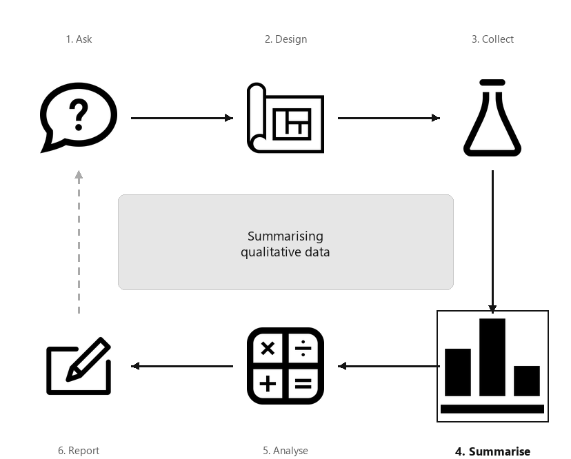
So far, you have learnt to ask an RQ, design a study, collect the data, classify the data, and summarise quantitative data In this chapter, you will learn to:
A diagram showing the six steps of research, arranged in a cycle: Ask, Design, Collect, Classify and summarise, Analyse, Report. Step 4 (Summarise) is highlighted, captioned “Summarising qualitative data”.
Many quantitative research studies involve qualitative variables. Except for very small amounts of data, understanding the data is difficult without a summary. As with quantitative data, qualitative data can be understood by knowing how often values of the variables appear. This is called the distribution of the data (Def. Definition 11.1).
The distribution can be displayed using a frequency table (Sect. Section 12.2) or a graph (Sect. Section 12.3). Qualitative data can be summarised by finding modes or, for ordinal qualitative data, using medians (Sect. Section 12.6). The distribution of qualitative data can be summarised numerically by computing proportions, percentages (Sect. Section 12.4) or odds (Sect. Section 12.5).
Qualitative data are typically collated in a frequency table. The rows (or the columns) should list the levels of the variable, and these should be exhaustive (cover all levels) and mutually exclusive (observations belong to only one level). The number of observations or the percentage of observations (or both) are then given for each level.
For nominal data, the levels of the variables can be displayed in alphabetical order, in order of size, in order of personal preference, or in any other order: use the order most likely to be useful to readers. For ordinal data, the natural order of the levels should almost always be used.
[103] surveyed \(400\) residents of Phoenix (Arizona) about their opinions of autonomous vehicles (AVs). Demographic information (Table Table 12.2) and respondents’ opinions of sharing roads with AVs (Table Table 12.3) were recorded.
The gender of the respondent is nominal (two levels), while the age group is ordinal (six levels). The levels are shown in the rows. The three questions about safety (Table Table 12.3) all yield ordinal responses (five levels, in columns).
Dot charts indicate the counts (or corresponding percentages) in each level using dots (or some other symbol). The levels can be on the horizontal or vertical axis, and the counts or percentages on the other. Placing the levels on the vertical axis often makes for easier reading, and space for long labels.
The axis displaying the counts (or percentages) should start from zero, since the distance of the dots from the axis visually implies the frequency of those observations (see Example Example 17.5).
Bar charts use bars to represent the number (or percentage) of observations in each level. As with dot charts, the levels can be on the horizontal or vertical axis, but placing the level names on the vertical axis often makes for easier reading, and room for long labels.
In contrast to bar charts, bars in histograms are butted together (except when an interval has a zero count), as the variable-axis usually represents a continuous numerical scale.
The axis displaying the counts (or percentages) should start from zero, since the height of the bars visually implies the frequency of those observations (see Example Example 17.5).
Consider studying the percentage of people who use Firefox, Chrome, and Safari as web browsers. A pie chart is not suitable for displaying the data, as people can use more than one of these browsers (i.e., the options are not mutually exclusive) nor exhaustive (i.e., other options exist).
In the pie chart (Fig. Figure 12.11, bottom left panel), determining which age groups have the fewest and most respondents is hard. The equivalent bar chart or dot chart makes the comparison easy. The tilted pie chart makes this comparison even harder (Fig. Figure 12.11, bottom right panel).
Recall that the purpose of a graph is to display the information in the clearest, simplest possible way, to facilitate understanding the message(s) in the data. A pie chart often makes the message hard to see [157].
Four panels showing the age group of AV study respondents: top left is a dot chart, top right is a bar chart, bottom left is a pie chart, and bottom right is a tilted (3D) pie chart.
Section12.4Numerical summary: proportions and percentages
Qualitative data can be summarised numerically by using the proportion or percentage of individuals in each level. These can be given instead of, or with, the counts (Tables Table 12.2 and Table 12.3).
Population proportions are almost always unknown. Instead, the population proportion (the parameter), denoted \(p\text{,}\) is estimated by a sample proportion (a statistic), denoted by \(\hat{p}\text{.}\)
As always, only one possible sample is studied. Statistics are estimates of parameters, and the value of the statistic is not the same for every possible sample.
Consider the AV data in Table Table 12.2, summarising results from a sample of \(n = 400\) respondents. The sample proportion of respondents aged \(25\) to \(34\) is \(76 \div 400\text{,}\) or \(0.19\text{.}\) The sample percentage of respondents aged \(25\) to \(34\) is \(0.19 \times 100\text{,}\) or \(19\)%, as in the table.
For the AV data in Table Table 12.2, the number of females is slightly larger than the number of males. Specifically, the ratio of females to males is \(204 \div 196 = 1.04\text{;}\) that is, there are \(1.04\)times as many females as males. This value of \(1.04\) is the odds that a respondent is female in the sample. An alternative interpretation is that there are \(1.04 \times 100 = 104\) females for every \(100\) males in the sample.
While proportions and percentages are computed as the number of results of interest divided by the total number, the odds are computed as the number of results of interest divided by the remaining number (Fig. Figure 12.17).
The odds are the number (or proportion, or percentage) of results of interest, divided by the remaining number (or proportion, or percentage) of results:
\begin{equation*}
\text{Odds} = \frac{\text{Proportion of results of interest}} {\text{Remaining proportion of results}} = \frac{\text{Percentage of results of interest}} {\text{Remaining percentage of results}}.
\end{equation*}
The odds are how many times the result of interest occurs compared to the number of times the results of interest does not occur.
A diagram comparing proportions and odds: the left side shows a fraction with the count of interest over the total, the right side shows the count of interest over the remaining count.
The AV data (Table Table 12.2) includes \(204\) females and \(196\) males. The odds that a respondent is female is \(1.04\text{.}\) The odds are greater than one, as there are more females than males. Alternatively, there are \(104\) females for every \(100\) males.
The odds that a respondent is male is \(196/204 = 0.96\text{;}\) there are \(0.96\)times the number of males as females. The odds are less than one, as there are fewer males than females. Alternatively, there are \(96\) males for every \(100\) females.
The percentage of respondents aged \(18\) to \(24\) is \(52/400 \times 100 = 13\)%. The odds that a respondent is aged \(18\) to \(24\) is \(52/(400 - 52) = 0.15\text{.}\) This means the number of respondents aged \(18\) to \(24\) is \(0.15\) times (i.e., less then) the number of respondents aged over \(24\text{.}\)
The odds that a respondent is aged \(18\) to \(54\) is \((52 + 76 + 76 + 72)/(56 + 68) = 2.23\text{.}\) This means the number of respondents aged \(18\) to \(54\) is \(2.23\) times (i.e., greater than) the number of respondents aged \(55\) or over.
The population odds (the parameter) are almost always unknown, and are estimated by the sample odds (the statistic). No symbol is commonly used to denote odds.
Section12.6Describing the distribution: modes and medians
Graphs are constructed to help readers understand the data, so any important features in the graph should be described. One simple way is to identify the level (or levels) with the most observations. This is called the mode.
Medians can be found for ordinal data (but not nominal data), since ordinal data have levels with a natural order. The median is the level in which the middle response is located, when the levels from all individuals are placed in order. The sample median estimates the unknown population median.
Consider the data in Tables Table 12.2 and Table 12.3. ’Gender’ is nominal qualitative, so medians are not appropriate. However, the other variables are ordinal, so medians could be used to describe each variable. Since \(n = 400\text{,}\) the median response will be halfway between the location of the \(200\)th and \(201\)st response when ordered:
Importantly, all these numerical quantities are computed from a sample (i.e., are statistics; Def. Definition 11.29), even though the whole population is of interest (i.e., the parameter; Def. Definition 11.28).
Means (Sect. Subsection 11.6.1) are generally not suitable for numerically summarising qualitative data. However, ordinal data may be numerically summarised like quantitative data in rare and very special circumstances. Means may be appropriate if both of these are true:
Qualitative variables should be summarised in a table. The table should include, as a minimum, numbers and/or percentages for each level. While useful in other contexts (see Chap. Chapter 15), odds are usually not given in the summary table. Examples are shown in Tables Table 12.2 and Table 12.3, and in the next section.
[119] recorded data about access to water for three rural communities in Cameroon (see Sect. Section 11.10). Numerous qualitative variables are recorded; some are displayed in Fig. Figure 12.24, and summarised in Table Table 12.25. Notice that the levels of the two ordinal variables are displayed in their natural order.
The distance to the nearest water source is usually less than \(1\) km, and the wait is often over \(15\) mins. The most common water source (i,e., the mode) is a bore (\(68.6\)%). The median (and mode) distance to the water source was \(100\) to \(1000\) m; the median wait time was \(5\) to \(15\) mins (the mode wait time was under \(5\) mins).
Three dot charts showing qualitative variables from the water-access study: distance to water source, queue wait time at water source, and type of water source.
Figure12.24.The distance to the water source (left), the wait time at the water source (centre), and the water sources (right) for the water-access study.
Qualitative data can be graphed with a dot chart, bar chart or (in special circumstances) pie chart. Qualitative data can be described using the mode or (for ordinal data only) a median. Qualitative data can be numerically summarised using proportions, percentages or odds.
[263] recorded the number of cylinders in many models of cars: eleven cars had four cylinders, seven cars had six cylinders, and fourteen cars had eight cylinders. The number of cylinders is quantitative discrete, but with so few different values, the data could be plotted with a graph used for qualitative data. For these data:
A survey of voice assistants (such as Amazon Echo; Google Home; etc.) conducted by Nielsen asked respondents to indicate how they used their voice assistant. The options were:
Respondents could select all options that applied. What would be the best graph for displaying respondents answers? Would a pie chart be suitable? Explain your answer.
[258] studied the taste of bread with varying salt and fibre content. Information was recorded from \(300\) subjects, including the subjects’ responses to the statement ’Rolls with lower salt content taste worse than regular ones’, on a five-point ordinal scale from ’Strongly Agree’ to ’Strongly Disagree’; see Table Table 12.28.
[119] asked \(231\) farmers what they considered to be the advantages and disadvantages of using reclaimed water on the farm. The responses are shown in Table Table 12.29 (not all farmers responded).
[264] studied \(284\) university students in Joinville, Brazil, tabulating how students got to campus (Table Table 12.30; each student could select one option only).
[Dataset: BabyBoom] The dataset shows the gender of \(44\) babies born in a hospital on one day [290][233]. The data are given in the order in which the births occurred.
[309] studied the influence of using ankle-foot orthoses in children with cerebral palsy. The data in Table Table 10.24 give the data for the \(15\) subjects. (Gmfcs is the Gross Motor Function Classification System used to describe the impact of cerebral palsy on their motor function; where lower levels mean better functionality.)