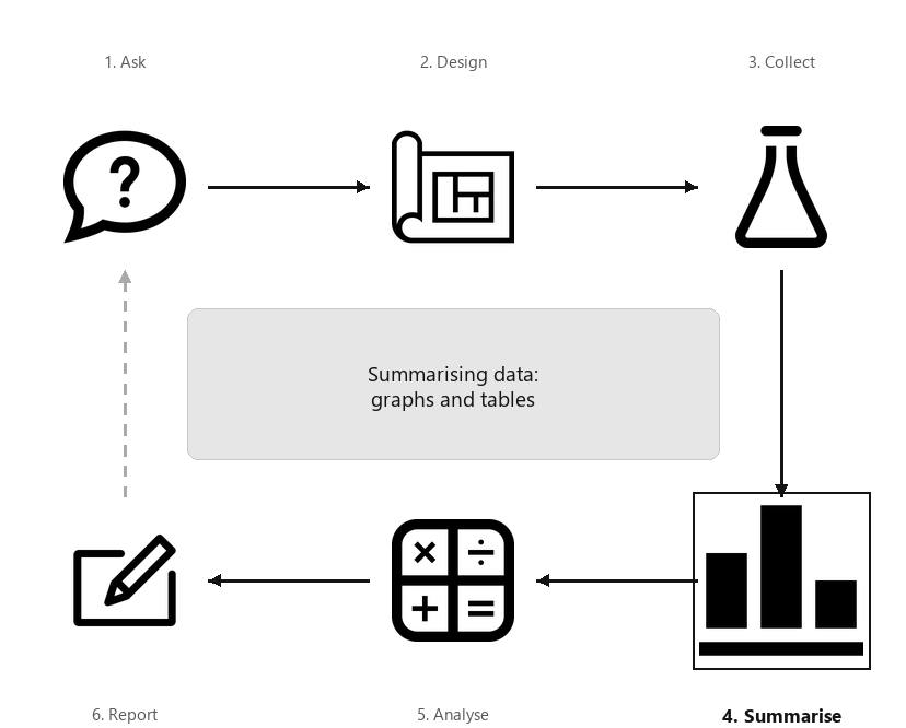
A diagram showing the six steps of research, arranged in a cycle: Ask, Design, Collect, Classify and summarise, Analyse, Report. Step 4 (Summarise) is highlighted, captioned “Summarising data: graphs and tables”.
A summary of the data is important for understanding the data, and for planning the direction of the analysis. In this chapter, we make some general comments for constructing graphs and tables. Always remember:
The purpose of a graph and a table is to display the information in the clearest, simplest possible way, to facilitate understanding the message(s) in the data.
Helping readers to understand the data is the goal of producing a graph. You should be able to sketch graphs by hand, but usually software is used to produce graphs. Using a computer makes it easy to try different graphs, to change features of graphs, and to produce the best graph possible. When creating graphs, ensure you:
Subsection17.2.1Avoid unnecessary third dimensions
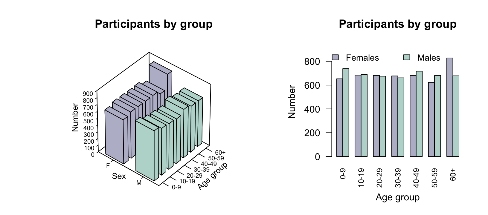
Graphs should focus on clear communication. One barrier to clear communication is using an unnecessary third dimension. This is poor: such graphs can be misleading and hard to read [157].
In the nhanes study [160], the age and sex of each participant were recorded. Using Fig. Figure 17.3 (left panel), can you easily determine if more females or more males are present in each age group?
The artificial third dimension makes determining the heights of the bars hard. In contrast, a side-by-side bar graph (Fig. Figure 17.3, right panel) makes it clear whether each age group has more females or more males.
Some plots, such as dot charts and scatterplots, may suffer from overplotting: when multiple observations have the same (or nearly the same) values, and these cannot be distinguished on the graph. Overplotting can especially be a problem when plotting discrete quantitative data. In many cases (such as dot charts), points can be jittered by adding a small amount of randomness to the observations, or stacked; see Example Example 14.7. Jittering is the best option for scatterplots. Overplotted points can change readers’ impression of the data, since some observations are obscured and are effectively ’lost’ to the reader.
One common optical illusion occurs when the frequency (or percentage) axis does not start at zero. This is a problem in graphs where the distance represented visually implies the frequency of those observations, as with the count (or percentage) axis in bar charts, dot charts, or histograms. This is not a problem in, for example, boxplots and scatterplots, where the distance of points from zero do not visually imply any quantity of interest.
Sometimes, the axes may be truncated intentionally so the differences are easier to see. In these cases, the reader should be alerted that the axes have been truncated for this reason.
The graph is visually misleading when the graph does not start at a count of zero, since the height of the bars from the axis visually implies the frequency of those observations.
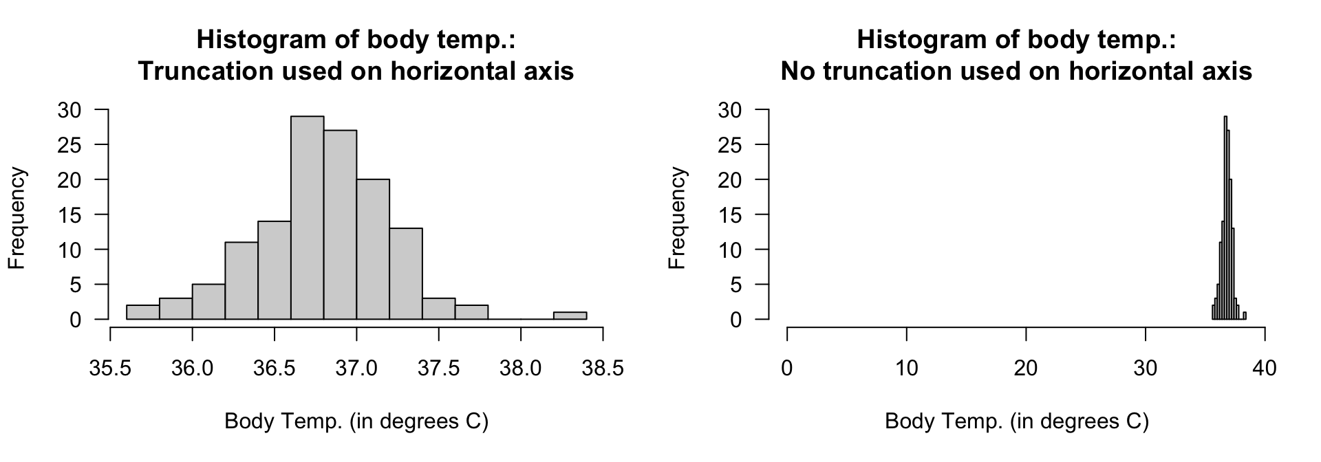
Consider data recording the body temperature of \(n = 130\) people ([34], [91]). A histogram of the data (Fig. Figure 17.9, left panel) clearly shows the distribution of body temperatures.
The vertical axis, displaying the counts, must start at zero since the bar heights visually imply a quantity of interest. However, the horizontal axis starts at \(35.5^{\circ}\text{C}\text{,}\) which does not create any problems as the distances from a temperature of \(0^{\circ}\text{C}\) do not visually imply any quantity of interest.
In contrast, starting the horizontal axis at a temperature of \(0^{\circ}\text{C}\) (Fig. Figure 17.9, right panel) makes any details in the histogram difficult to see; the histogram is pointless.
As noted in Sect. Subsection 12.3.3, pie charts may be hard to read: humans compare lengths (bar and dot charts) better than angles (pie charts) [159]. Pie charts are also difficult to use with levels having zero or small counts.
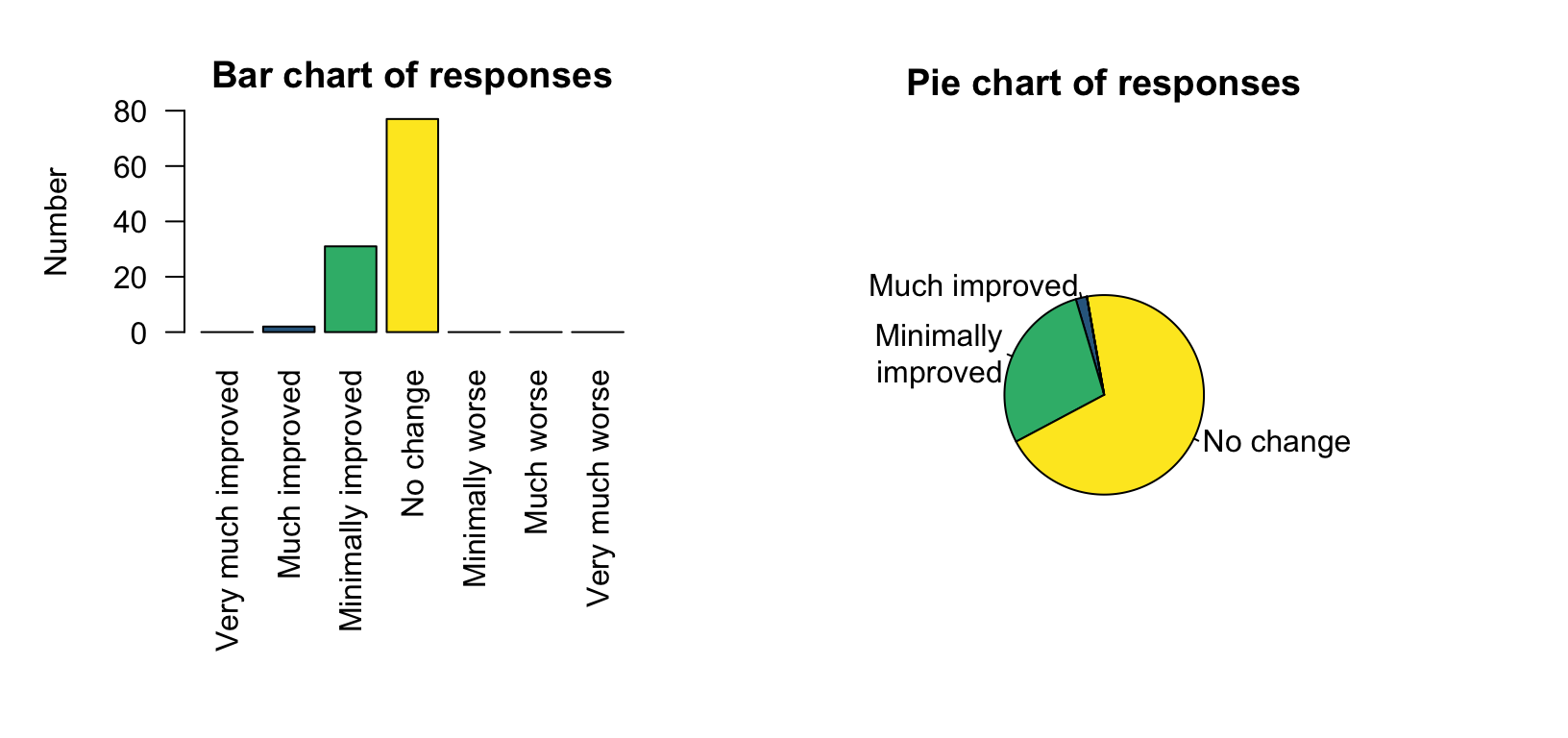
[161] studied the use of ginkgo for memory enhancement. Caregivers blinded to the treatment (ginkgo or placebo) reported the impact on subjects’ memory. The bar chart (Fig. Figure 17.7, left panel), for subjects on the placebo, shows that four of the available categories had zero responses, and one had a very small number of responses (two). The pie chart (right) make the small category difficult to see, and the categories with zero counts impossible to see.
Figure17.7.Data with zeros and small counts are easy to see in a bar chart (left panel) and dot chart, but difficult to see in a pie chart (right panel).
A computer is helpful for constructing tables. Using a computer also makes it easy to try different orientations or layouts. As with graphs, the purpose of tables is to help readers understand the data. When creating numerical summary tables, ensure you:
do construct the table to allow readers to easily make the important comparisons, as far as possible (space restriction may take precedence, for example).
do not use vertical lines (in general), and use very few horizontal lines. Horizontal lines can be used to group columns (for example, see Table Table 17.8).
[119] recorded data about access to water in three rural communities in Cameroon (see Sects. Section 12.8 and Section 11.10). The study could be used to determine associations to the incidence of diarrhoea in young children (\(85\) households had children under \(5\) years of age). Relationships between the incidence of diarrhoea and some other variables appear in Figs. Figure 15.24 and Figure 14.16. A summary table of information can also be constructed (Table Table 17.8).
Table17.8.Numerical summary of the water-access data in \(85\) households with children, according to whether children under \(5\) years of age had reported diarrhoea in the last two weeks.
Since the observed sample is one of countless possible samples that may have been selected, answering RQs about the population is not straightforward. In the observed sample, \(85.0\)% of households that did not keep livestock reported diarrhoea in children under \(5\text{,}\) while \(64.6\)% of households that did keep livestock reported diarrhoea in children under \(5\text{.}\) That is, a difference is seen in the sample; but RQs ask about the population.
The sample percentages are different simply because of the households selected in this particular sample. Another sample, with different households, might produce different sample percentages. Sampling variation explains the difference in the sample percentages.
The difficulty is knowing which of these reasons (’hypotheses’) is the most likely explanation for the difference between the sample percentages. This question is of prime importance as it answers the RQ. Tools for answering these questions are considered later in this book.
Researchers record the pH of water and the temperature of the water, in various creeks in the north island of New Zealand, to explore the relationship between pH and temperature.
[151] recorded these variables for \(385\) lime trees in Russia: the foliage biomass (in kg; the response variable); the tree diameter (in cm; the explanatory variable); the age of the tree (in years); and the origin of the tree (one of Coppice, Natural, or Planted).
The purpose of the study is to estimate the foliage biomass from the tree diameter, in the presence of some extraneous variables. What graphs would be useful?
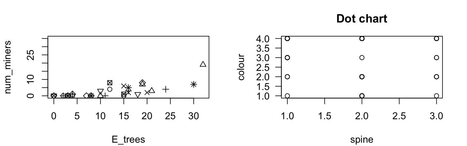
[162] counted the number of noisy miners (an Australian bird) and eucalyptus trees in random quadrats. Critique the graph (not given by [162]!) of the data (Fig. Figure 17.10, left panel).
[163] recorded, among other variables, the colour of the carapace (’Light medium’, ’Medium’, ’Dark medium’ or ’Dark’) and the condition of the carapace (’Both OK’, ’One OK’, ’None OK’) of \(n = 173\) female horseshoe crabs. Critique the scatterplot (Fig. Figure 17.10, right panel) used to explore the data.
[165] examined the change in madrs (a quantitative scale measuring level of depression) and treatment group (whether each person was treated using: exercise; body awareness; or advice).
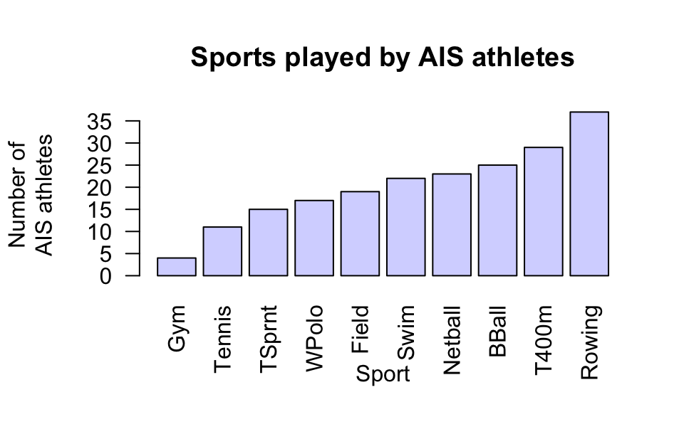
A study of high-performance athletes at the Australian Institute of Sport (AIS) [126] recorded numerous variables about athletes. A plot for the sports played by the athletes is shown in Fig. Figure 17.11. How would you describe the data: left skewed, right skewed, approximately symmetrical? Or something else?
[Dataset: Typing] The Typing dataset [69] contains four variables: typing speed (mTS), typing accuracy (mAcc), age (Age), and sex (Sex) for \(1\,301\) students. Produce graphs necessary for understanding the data, making sure to explain what they reveal.
Does the mean typing speed or mean accuracy appear to differ by the age or sex of the student? What other questions could be useful to ask about the data?
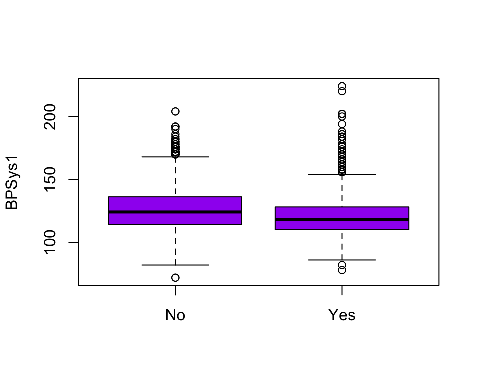
[Dataset: NHANES] Consider the nhanes data. In preparing a paper about this study, suppose Fig. Figure 17.13 and Tables Table 17.12 were produced. Critique these.
Figure17.9.Two histograms displaying the body temperature of \(130\) people. Left: a well-constructed histogram. Right: a poorly-constructed histogram.
Figure17.10.Left: the number of noisy miners and the number of eucalyptus trees. Right: a scatterplot of the colour of female horseshoe crabs and the condition of their spines.