Chapter 34 Selecting an analysis

Objectives

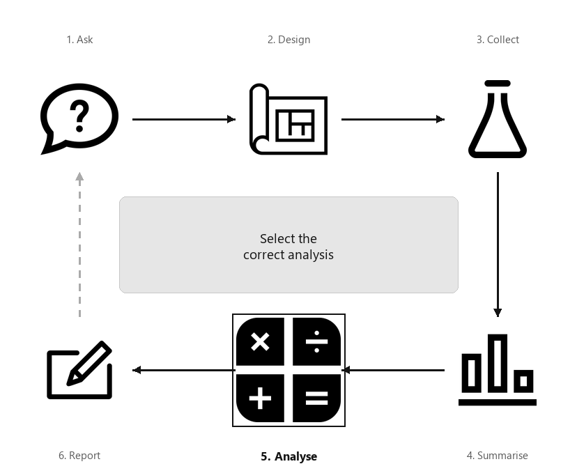
So far, you have learnt about the research process, including analysing data using confidence intervals and conducting hypothesis tests. In this chapter, you will learn to:

select the correct analysis.

A diagram showing the six steps of research, arranged in a cycle: Ask, Design, Collect, Classify and summarise, Analyse, Report. Step 5 (Analyse) is highlighted, captioned “Select the correct analysis”.

Section 34.1 About selecting an appropriate analysis

Selecting the correct CI or hypothesis test can be challenging, and this book only describes a few possible scenarios. For the situations studied in this book, identifying the type of RQ (e.g., descriptive or correlational), and the number and type of variables (qualitative or quantitative) is important (Table Table 34.1). The Appendix may also prove useful.

Table 34.1. Analysis scenarios studied

Summaries		Analysis
Graphical display	Numerical summary	Confidence interval	Hypothesis test
Descriptive RQ: proportion in one sample (i.e., one qualitative variable)
Bar charts; pie chart	Counts; percentages; odds	CI for one mean 22	One-sample \(z\)-test 26
Descriptive RQ: mean of one sample (i.e., one quantitative variable)
Histogram; stemplot; dot chart	Means, medians; std dev., IQR; outliers	CI for one mean 23	One-sample \(t\)-test 27
Repeated-measures RQ: paired quantitative data
Histogram of differences 13.3.1; case-profile 13.3.2	Mean, std dev. etc. of differences	CI for mean difference 29	\(t\)-test for mean differences 29
Relational RQs: comparing quantitative variables
Error bar chart 30.2	Mean and std error of the difference; mean, std dev. etc. of each group	CI of the difference between two means 30	\(t\)-test for the difference between two means 30
Relational RQs: comparing qualitative variables
Side-by-side bar chart; stacked bar chart	Odds; OR; percentages	CI for ORs; CI for difference between two proportions 31	\(\chi^2\)-test for OR; \(z\)-test for difference between two proportions 31
Correlational RQs
Scatterplot	Correlation coefficient; \(R^2\)	CI for correlation coefficient; CI for regression parameters 33	Test for correlation; \(t\)-test for regression parameters 33

Example 34.2. Selecting an analysis.

[188] studied whether the ’presence of a prehospital physician improves survival from cardiac arrest’ (p. 227). They studied 471 cardiac arrests: \(200\) treated by prehospital physicians (2004 to 2007), and \(271\) treated by emergency medical technicians (2008 to 2014).

For each cardiac admission (the unit of analysis), two variables are recorded. Whether a prehospital physician is present (the explanatory variable) is qualitative with two levels (Yes; No). Whether a patient survived (the response variable) is qualitative with two levels (Yes; No). They compared the survival proportions for the two scenarios; this is a relational RQ.

To study the proportion of survivors for each scenario, a \(z\)-test for the difference between proportions (and corresponding CI) would be used. Alternatively, a \(\chi^2\)-test for comparing the odds of survival (and a CI for the OR) could also be used.

Example 34.3. Selecting an analysis.

[281] studied the relationship between the ball release speed (BRS) and the height of female cricket players, and BRS and arm length. Since they are exploring the relationship between two pairs of quantitative variables, both RQs are correlational RQs.

If the relationships are approximately linear (determined by examining the two scatterplots), a test for correlations (and corresponding CI) would be used, for one each relationship to be studied. Alternatively, a linear regression model could be fitted (one for each relationship), and a test for the slope of the fitted regression equation (and corresponding CI) could be conducted.

Example 34.4. Selecting an analysis.

[266] studied the impact of soil lead levels in New Orleans (USA) neighbourhoods on northern mockingbirds (p. 2):

We tested the hypothesis that nestling mockingbird lead levels in blood and feathers differ with respect to neighborhood soil lead levels...

They compared the mean lead concentration in blood, for birds in neighbourhoods with low and with high lead levels. They also compared the mean lead concentration in feathers, for birds in neighbourhoods with low and high lead levels. These are both relational RQs.

For each bird (the unit of analysis), three variables were recorded. The lead levels (the explanatory variable) is qualitative with two levels: high lead-level neighbourhoods, and low lead-level neighbourhoods. The blood lead concentrations (one response variable) is quantitative (continuous). The lead concentrations in feathers (another response variable) is quantitative (continuous).

To study the difference between the mean lead concentrations in the two groups, a two-sample \(t\)-test for the difference between the means (and the corresponding CI) is needed (provided the statistical validity assumptions are met). One test is needed for comparing blood lead concentrations, and another for comparing concentrations in feathers.

The following short video may help explain some of these concepts. Note that the test for correlation and regression have not yet been covered in this book (but they will be in the next few chapters).

Exercises 34.2 Exercises

Answers to odd-numbered exercises are given at the end of the book.

1.

Identify which of these statistics do not have a sampling distribution well-modelled by a normal distribution. Explain your answer.

The difference between two sample means \(\bar{x}_1 - \bar{x}_2\text{,}\) with samples of size \(n_1 = 55\) and \(n_2 = 61\text{,}\) but slightly right-skewed distributions of the data for each sample.
The sample slope in a regression equation \(b_1\text{,}\) with an approximate linear relationship between the variables, approximately constant variation in the values of \(y\text{,}\) and \(n = 24\text{.}\)
The sample OR, with both samples of size \(n = 43\text{.}\)

2.

Identify which of these statistics do not have a sampling distribution well-modelled by a normal distribution. Explain your answer.

The sample mean of a set of differences \(\bar{d}\text{,}\) with a sample of \(n = 32\) difference, but the distribution of the differences are slightly right-skewed.
The sample correlation coefficient \(r\text{,}\) with an approximate linear relationship between the variables, approximately constant variation in the values of \(y\text{,}\) and \(n = 29\text{.}\)
The sample proportion \(\hat{p}\text{,}\) with \(n = 26\) and \(\hat{p} = 0.154\text{.}\)

3.

Suppose researchers compare the mean number of hours of exercise per week for the same British office workers, both in summer and in winter, to study the mean change.