So far, you have learnt the about the process of research: asking an RQ, designing a study, collecting data, describing and summarising the data, and analysing the data. You have learnt how to write about your research. In this chapter, you will learn to:
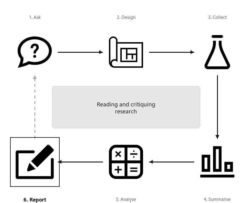
A diagram showing the six steps of research, arranged in a cycle: Ask, Design, Collect, Classify and summarise, Analyse, Report. Step 6 (Report) is highlighted, captioned “Reading and critiquing research”.
All academic disciplines change and adapt. Staying current in your discipline requires reading, critiquing and understanding the research of others, as communicated in journal articles or presentations (Chap. Chapter 35). (Critiquing means to evaluate: identifying what is good, and what can be improved.)
Familiarity with the language and concepts of research is important for understanding these articles, even if you will not be conducting your own research.
Reading research articles can be challenging. Rather than reading articles thoroughly from start to finish, first read the Abstract to obtain an overview of the whole article, without becoming lost in the details. Then, read the Discussion, which highlights the important findings. Next, skim the rest of the article (perhaps focusing on graphs and tables of results). Finally, if necessary, read the article for details.
Terminology and notation varies widely in research (Sect. Subsection 35.6.3). When reading research, check the terminology and notation being used if you are unsure!
[301] studied the impact of texting (on a smartphone) on how students walk (including walking speed). In this section, the article will be briefly discussed.
The aim of this experiment was to investigate whether using a cell phone while walking affects walking velocity […] in young people. Forty-two subjects (\(20\) males, \(22\) females; mean age: \(20.74\pm 1.34\) years; mean height: \(173.21\pm 8.07\) cm; mean weight: \(69.05\pm 14.07\) kg) participated in the study. The subjects were asked to walk on an FDM–1.5 dynamometer platform four times at a constant comfortable velocity and a fast velocity of their choice. They were asked to continuously type one sentence on a cell phone while walking at the same velocity. The results showed that texting while walking led to a significant reduction in velocity compared to walking without the phone.
As this is the abstract, many details are absent (but explained in the article itself). Nonetheless, a lot can be learnt about the study from the abstract.
a quantitative variable (walking velocity) is being compared within individuals, so paired \(t\)-tests are a likely method of analysis (Chap. Objectives 29).
... to analyze how the use of a cell phone while walking at different velocities affects gait parameters, i.e., velocity, cadence, stride width, and stride length.
The sample comprises students from the University School of Physical Education (Poland) studying a course in gait analysis. This sample may not represent any general population, though the conclusions may possibly apply to non-students and not-Poles.
Control variables included the temperature and humidity: ’the air temperature was constant at \(22\) degrees Celsius, and the air humidity was \(47\)%’ (p. 3).
Five response variables were used: left-side stride length, right-side stride length, cadence, stride width, and walking velocity. These appear to have been measured objectively.
The data are not immediately available (probably due to ethics concerns) but ’are available upon request’ (p. 7). Details of the analysis were not available.
Case-profile plots were produced for the five response variables, showing the means for each task rather than for all \(42\) individuals (much like Fig. Figure 13.23).
Correlations were computed between the five response variables. The correlations between stride width and the other variables were negative; all other correlations were positive. Since the relationships were non-linear, Spearman correlations were used rather than the Pearson correlations studied in Chap. Chapter 33. All the corresponding \(P\)-values were less than \(0.05\) apart from the correlation between stride width and cadence.
The mean and standard deviation of the three response variables were provided for each task. However, the numerical summary for the differences were not provided; a \(P\)-value only was provided.
Fifteen hypothesis tests were conducted: the three between-tasks comparison above, for the five response variables. This increases the chance of making a Type I error.
’Statistically significant’ was defined as a \(P\)-value smaller than \(0.017\text{,}\) rather than the commonly-used \(P < 0.05\text{.}\) The reason was to reduce the chance of making a Type I error (Sect. Section 28.7), but the details are beyond the scope of this book.
... right and left single step length and gait velocity, were found to be statistically significant in each comparison. The value of the change in step width was statistically significant only when comparing trials 1 and 3, and cadence showed statistical significance when comparing trials 2 and 4, as well as 3 and 4.
The researchers also made qualitative observations; they observed ’moments when the subject took their eyes off the phone in order to assess the direction of the path’ (p. 5).
The researchers concluded that ’the use of a cell phone while walking significantly affects gait parameters, causing a decrease in walking velocity and a reduction in stride length’ (p. 6), thus providing answers to the RQs.
The researchers state (p. 6) that ’This proves that texting on a cell phone has a major impact on gait’. However, the research does not prove anything based on one of countless possible samples.
The study had poor ecological validity, as the study ’was conducted in a measurement workshop room, the air temperature was constant at 22 degrees Celsius, and the air humidity was 47\%’.
that the sentence typed by the subjects was unchanged in both Trials 3 and 4; hence, Trial 4 may have been easier than the previous trial as the sentence was familiar (the carryover effect).
that the step width differed between comfortable walking speed and walking at the same speed with the phone. The researchers attribute this to the carryover effect, as ’walking with the phone at comfortable velocity and at fast velocity directly followed one after the other’, and so ’subjects were able to respond to the new conditions by adapting to them during the first transition’.
The six steps of research can be used as a scaffold for critiquing research articles. Starting by reading the Abstract (or Summary, or Overview) for an overview, then the Discussion, and then skim the rest of the article (perhaps focusing on graphs and tables of results). If necessary, read the article for details.
... were recruited through word of mouth and posters displayed around the [researcher’s] university. Participants were eligible if they were ambulatory, \(\ge 18\) years of age, and owned an iPhone 6 […] or newer model.
Among many other comparisons, the researchers compared the mean difference between the number of step counts recorded by manually counting steps (mean: \(92.6\)) and the iPhone-recorded number of steps (mean: \(85.4\)). What statistical test would be appropriate?
While walking at \(2.5\kms\text{.h}^{-1}\text{,}\) the above statistical test resulted in \(t = 2.95\text{.}\) What is the approximate \(P\)-value? Interpret the results.
[100] studied the relationship between hearing loss, and headphone and earphone use in Iranian students, using a non-directional study. The article states:
Only \(866\) of the \(890\) students agreed to participated in the study; of these, \(745\) used earphones. The participants completed a hearing test and a Hearing Loss Questionnaire (HLQ; values between \(17\) and \(34\text{;}\) higher scores indicating more severe hearing loss).
Perform a hypothesis test to compare the difference between the mean hearing loss score for students who use and do not use earphones, and confirm that the \(P\)-value is indeed very small.
... \(1000\) cases of pregnant women living in urban and rural areas of Varzaghan city that consisted of \(550\) pre-earthquake and \(450\) post-earthquake cases.
The researchers compared the mothers in the two groups (pre- and post-earthquake) on various measurements. For example, the mean age of mothers in the pre-group was \(25.82\) y, and the mean age of the mothers in the post-group was \(26.71\) y; the difference has a \(P\)-value of \(0.084\text{.}\)
The researchers also compared the mean birth weights of the babies born to the mothers in the two groups. In the pre-group, the mean birth weight was \(3.25\kgs\) (\(s = 0.52\)) and in the post-group the mean birth weight was \(3.18\kgs\) (\(s = 0.54\)).
The researchers also compared the percentage of babies with a Low Birth Weight (LBW; less than \(2.5\kgs\)). For the pre-group, the percentage was \(6.01\)%; for the post-group, the percentage was \(8.92\)%.
[312] studied the selenium (Se) concentration in irrigation and stock water sources in California. For drinking water, the maximum recommended concentration was \(10\microgs.\xLs^{-1}\text{;}\) for irrigation water, the maximum recommended concentration was \(20\microgs.\xLs^{-1}\text{.}\)
Part of the study examined the area within \(5\kms\) of wells. When Pliocene rocks were within this radius, the relationship between the Se concentration \(y\) in the water and the electrical conductivity of the water \(x\) (in deciSiemens per meter, \(\text{dS.m}^{-1}\)) was \(\hat{y} = -3.1 + 7.0x\text{,}\) where \(R^2 = 27\)%.
[299] compared the larvae of two types of mosquitoes: Ae. albopictus (invasive) and Cx. pipiens (native). One study compared the survival rates of the larvae at two temperatures, and in the presence or absence of predator (a small crustacean, called copepods).
At \(15\)^o^C and \(25\)^o^C, the survival rates were \(86.8\)% and \(86.1\)%, respectively, for the control group (i.e., no copepods). The papers quoted a \(P\)-value of \(P = 0.8076\text{.}\)
The researchers also compared the size of the surviving larvae in the control groups for both temperatures. In comparing Cx. pipiens to Ae. albopictus larvae, the paper gives this information:
Megacyclops viridis (a copepod) preys on the larvae. The association between predation efficiency (\(y\text{;}\) a percentage) and predator–prey size-ratio (\(x\text{;}\) no units) was (using \(n = 45\)) \(\hat{y} = -19.56 + 31.64x\text{.}\) The standard errors of the regression coefficients were \(17.92\) (intercept) and \(13.88\) (slope).
[245] compared tomatoes growing on conventional (CNV; \(n = 14\)) and organic (ORG; \(n = 17\)) farms. Between 1989 and 1990, the researchers sampled tomato fields during April and September (p. \(1 100\)). An area between \(0.04\) and \(0.1\has\) was set aside within each field for collecting data. Each area was divided into \(20\) sections, then a \(1\ms\) row was selected at random within each section to be sampled.
Thus, two groups were used: one using eye-masks and earplugs (treatment group, \(T\text{;}\)\(n = 29\)) and one using sham headbands (control or placebo group, \(P\text{;}\)\(n = 27\)).
Sleep duration was measured in Week 1 (no intervention) and again in Week 2 (with the allocated intervention) for each subject, using a ’wrist actigraphy monitor’.
The women in the two groups were compared. For example, the mean age of the women was \(30.6\) y (\(s = 3.6\)) (\(T\)) and \(30.1\) y (\(s = 3.3\)) (\(P\)); the \(P\)-value for the comparison was given as \(P = 0.56\text{.}\)
Another comparison was the room ’condition’ where the women slept: in the treatment group, \(13\) had a room with a fan (\(16\) had air conditioning), while in the control group \(10\) women had a fan (and \(17\) air conditioning). The \(P\)-value for the comparison was given as \(P = 0.60\text{.}\)
In the treatment group, the mean sleep duration in Week 1 was \(279.0\mins\) (\(s = 18.9\)) and in Week 2 was \(303.6\mins\) (\(s = 18.8\)). The increase was \(24.7\mins\) (\(s = 14.9\)).
In the control group, the mean sleep duration in Week 1 was \(286.3\mins\) (\(s = 20.9\)) and in Week 2 was \(301.9\mins\) (\(s = 21.8\text{;}\)\(n = 26\)). The increase was \(18.1\mins\) (\(s = 17.3\)).
Table36.3.Number of wells with dissolved selenium (Se) concentration above \(2\microgs.\xLs^{-1}\text{,}\) and the geology within \(5\kms\) radius of the well.