So far, you have learnt to ask an RQ, design a study, classify and summarise the data, and construct some confidence intervals. In this chapter, you will learn more about forming confidence intervals. You will learn to
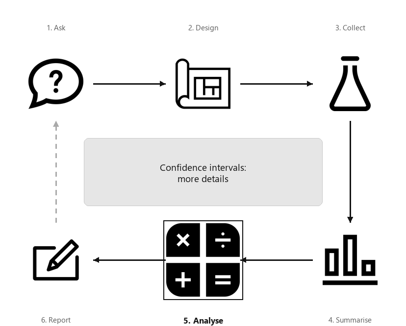
A diagram showing the six steps of research, arranged in a cycle: Ask, Design, Collect, Classify and summarise, Analyse, Report. Step 5 (Analyse) is highlighted, captioned “Confidence intervals: more details”.
The previous chapters discussed forming confidence intervals (CIs) for estimating a population proportion, and for estimating a population mean. CIs will also be studied (Chaps. Objectives 29 to Introduction 31) in other contexts. This chapter discusses some principles that apply to CIs in general:
CIs are formed for an unknown value of a population parameter (such as the population proportion \(p\)), using the best estimate: the value of the sample statistic (such as the sample proportion \(\hat{p}\)). When the sampling distribution of the statistic has an approximate normal distribution (and not all sampling distribution do have a normal distribution), CIs have the form
When the sampling distribution has an approximate normal distribution, the approximate\(95\)% CI uses a multiplier of \(2\) (from the \(68\)–\(95\)–\(99.7\) rule). To compute CIs other than \(95\)% CIs (such as \(99\)% CIs), and for exact\(95\)% CIs, software is used.
Confidence intervals (CIs) tell us about the unknown value of the population parameter, based on what we learn from one of the countless possible sample statistics.
Section24.2More details about statistical validity
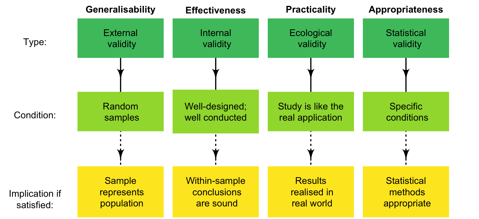
When CIs are computed, statistical validity conditions must be true to ensure the mathematics behind the calculations are sound. For instance, many CIs assume the sampling distribution has a normal distribution (so that, for example, the \(68\)–\(95\)–\(99.7\) rule can be used); the statistical validity conditions state the conditions under which the sampling distribution has an approximate normal distribution. If these conditions are not met, the sampling distribution may not be close to an approximate normal distribution, so the \(68\)–\(95\)–\(99.7\) rule (on which the CI is based) may not be appropriate, and the CI itself may be inappropriate. Of course, if the statistical validity conditions are close to being satisfied, then the resulting CI will still be reasonably useful.
Besides checking the statistical validity conditions, the internal validity and external validity of the study should be discussed (Fig. Figure 24.2). In addition, CIs also require that the sample size is less than about \(10\)% of the population size; this is almost always the case.
If the CI is an approximate CI (e.g., based on using an approximate multiplier of \(2\) from the \(68\)–\(95\)–\(99.7\) rule), this should also be clear.
The sample mean cadmium concentration of peanuts is \(0.0768\ppms\) (\(n = 290\)), with an approximate \(95\)% CI from \(0.0714\) to \(0.0822\ppms\text{.}\)
That is, if we repeated the process (of selecting a sample of a given size, then computing the CI) numerous times, \(95\)% of those CIs formed would contain the value of the parameter. This is the idea shown in the animation in Sect. Section 22.5.
In practice, this definition is unsatisfying, since we only ever have one sample, not many samples. Furthermore, since the value of the parameter is unknown (after all, the reason for taking a sample was to estimate the value of the parameter), we don’t know if the CI from our single sample straddles the population parameter or not.
The \(95\)% CI gives a range of values of the parameter that could reasonably (with \(95\)% confidence) have produced the observed value of the statistic.
Frequently, the CI is described as having a \(95\)% chance of containing the population parameter. This is not strictly correct (the CI either does or does not contain the value of the population parameter), but is a common and a brief paraphrase for the correct interpretation above.
I use this analogy: most people say the sun rises in the east. This is incorrect; the sun doesn’t rise at all. People say the sun rises in the east as a convenient way to explain that we see the sun each morning in the east as the earth rotates. Similarly, most people say a CI is an interval with a certain chance of containing the value of the population parameter, as a convenient way to explain the CI.
In Example Example 24.3, the approximate \(95\)% CI for the cadmium concentration in peanuts was from \(0.0714\) to \(0.0822\ppms\text{.}\) The correct interpretation is:
If many samples of \(290\) peanuts were taken, and the approximate \(95\)% CI computed for each one, about \(95\)% of those CIs would contain the population mean.
The range of values of \(\mu\) that could plausibly (with \(95\)% confidence) have produced \(\bar{x} = 0.0768\) is between \(0.0714\) to \(0.0822\ppms\text{.}\)
Confidence intervals (or CIs) tell us about the unknown population parameter, based on what we learn from one the countless possible sample statistics. CIs give an interval in which a parameter is likely to lie over repeated sampling. Since we only ever have one sample, two reasonable alternative interpretations for a \(95\)% CI are:
the \(95\)% CI gives a range of values of the parameter that could reasonably (with \(95\)% confidence) have produced our observed value of the statistic.
[265] computed a \(95\)% CI to estimate the proportion of trees with apple scab, and found \(\hat{p} = 0.314\) and \(s.e.(\hat{p}) = 0.091\text{.}\) What would be wrong with the following conclusions?
[16] studied the snacking habits of Australian children. In 2007 (for which \(n = 3\,637\)), the CI for the proportion of children snacking (’an eating occasion that occurred between meals based on time of day’; p. 1) was \(0.981\pm 0.003\) in 2007. What would be wrong with the following conclusion?
[219] studied how far amputees could walk in two minutes following a femoral (leg) implant. After \(14\) months, the sample of ten amputees walked a mean of \(122.5\ms\text{;}\) the \(95\)% CI was computed as \(96.4\ms\) to \(148.6\ms\text{.}\) What would be wrong with the following conclusions?
A study of sodium intake in Thailand found the \(95\)% CI for the mean daily sodium intake for subjects with a secondary school education was \(3\,565\) to \(3\,903\mgs\text{.}\) What would be wrong with the following conclusions?
The average adult male Leadbeater’s possum weighed \(137\gs\) (\(95\)% CI = \(135\gs\text{,}\)\(139\gs\)), with \(90\)% of weights between \(122\) and \(153\gs\text{.}\)
Figure Figure 22.15 indicates that a higher value for the confidence level means wider CIs, since wider intervals are needed to be more certain that the interval contains the value of the parameter that produced the value of the statistic.