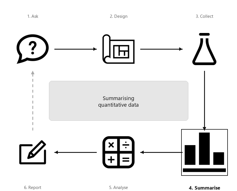
A diagram showing the six steps of research, arranged in a cycle: Ask, Design, Collect, Classify and summarise, Analyse, Report. Step 4 (Summarise) is highlighted, captioned “Summarising quantitative data”.
Many quantitative research studies involve quantitative variables. Except for very small amounts of data, understanding the data is difficult without a summary. Quantitative data can be summarised by knowing how often various values of the variable appear. This is called the distribution of the data.
The distribution can be displayed using a frequency table (Section 11.2) or a graph (Section 11.3). The distribution of quantitative data can be described by the shape (Section 11.5), and summarised numerically by computing the average value (Section 11.6), computing the amount of variation (Section 11.7), and identifying outliers (Section 11.8).
Quantitative data can be collated in a frequency table by grouping the variables into appropriate intervals (’bins’). The intervals should be exhaustive (cover all values) and mutually exclusive (observations belong to one and only one category). While not essential, usually the categories have equal width.
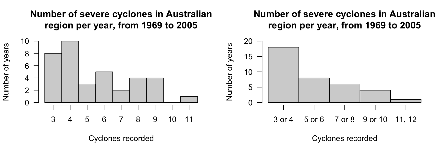
A frequency table can be constructed by binning each discrete value individually (Table 11.4, left table) or grouped in pairs (Table 11.4, right table). The table gives the number of years, and the corresponding percentages, that recorded the given number of cyclones.
For continuous data, care is needed when creating frequency tables. Bins must be carefully constructed, since all continuous data are rounded. The bins should be defined to ensure no values lie on the border between bins, and hence creating ambiguity.
Table 11.6 gives the weights of babies born in a hospital on one day [290][233], plus the gender of each baby, and the number of minutes after midnight of the birth (shown in birth order).
To display the distribution of birth weights, the weights can be grouped into clearly-defined weight intervals (Table 11.7, left column). Alternatively, the breaks between the bins can be given to one more decimal place than the data to avoid observations landing exactly on the bin divisions (final column).
The table also gives percentage of births in each bin; for example, the percentage of babies over \(4.0\) is \(1/44 100 = 2.27\)%, or about \(2\)%. Most babies in the sample are between \(3\) and \(4\) at birth.
Table11.6.The first nine observations (of \(n = 44\)) of the baby-births data: the number of babies born in a Brisbane (Australia) hospital on one specific day. The ‘birth time’ is the number of minutes after midnight.
Table11.7.The baby-weights data, displayed in a frequency table. The first and last columns show two different (but equivalent) ways to group the data.
Sometimes trial and error is needed to find useful intervals for continuous data. Usually, but not universally, the intervals include values at the lower end of the interval, but exclude values at the upper end (as in Table 11.7).
The graphs in this section are appropriate for continuous quantitative data, and sometimes for discrete quantitative data if many values are possible. Sometimes, discrete data with very few recorded values are better displayed using graphs designed for qualitative data (Section 12.3).
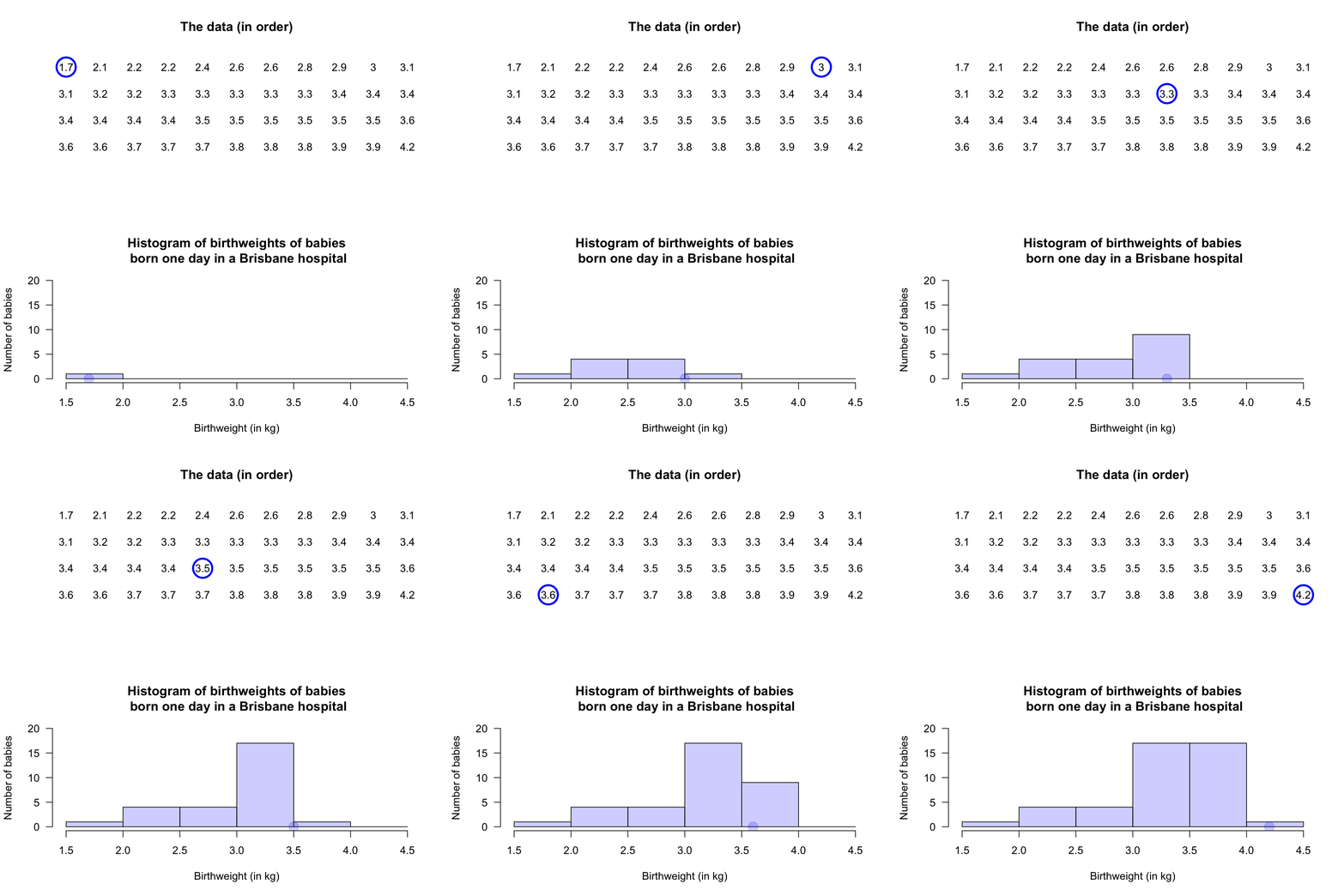
Histograms are a series of boxes, where the width of the box represents an interval of values of the variable being graphed, and the height of the box represents the number (or percentage) of observations within that range of values. 1
Actually, the area of the box is proportional to the number of observations. We only consider histograms where the boxes have the same width, so the statements are equivalent.
The height of the histogram bars indicate the number (or percentage) in each category (often called ’bins’). A histogram is essentially a picture of a frequency table. The vertical axis can be counts (labelled as ’Counts of trees’, ’Number of frogs’, ’Frequency of people’, or similar) or percentages.
The axis displaying the counts (or percentages) should start from zero, since the height of the bars visually implies the frequency of those observations (see Example 17.5).
When the quantitative variable is continuous, care is needed when constructing the histogram. Since the data are continuous, the data must be rounded. (For instance, the birthweights in Table 11.7 are rounded to one decimal place of a kilogram.) This means care is needed when defining boundaries between bins, and ensuring clarity about which bin contains observations when they lie on (or near) a boundary. One way to do this is to define the boundaries between bins to one more decimal place than the given data (as in the final column of Table 11.7).
The choice of bin size and bin boundaries can substantially change how a histogram displays the data (Examples Example 11.13 and Example 11.18). For large datasets, these choices tend to matter less.
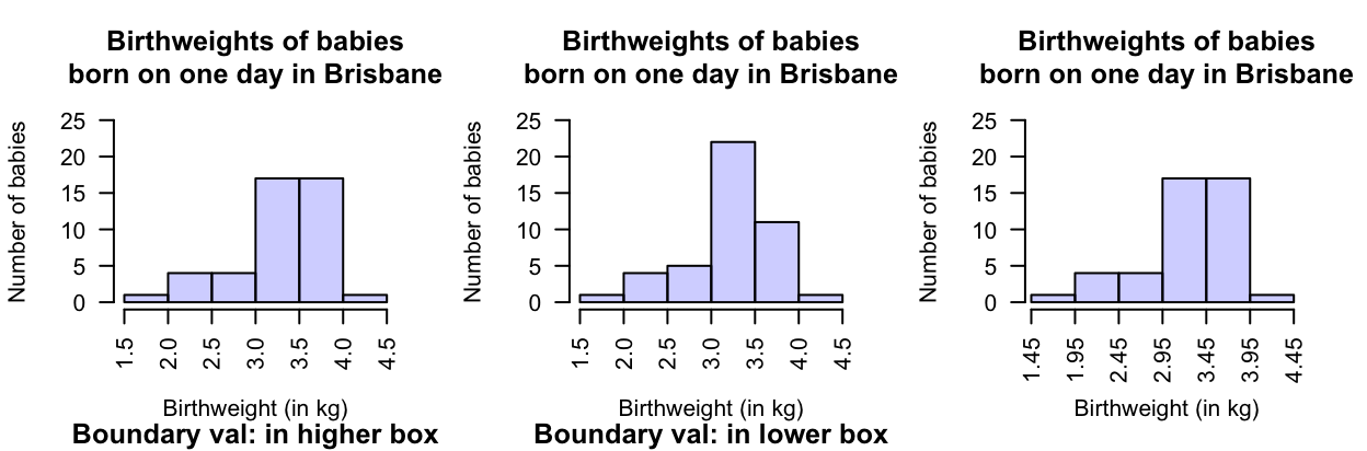
When observations lie on the boundary of the boxes, some software includes these observations in the lower box (which is common) and some in the higher box.
An observation on a boundary between the bins may be placed in the higher box (i.e., \(2.5\) is in the ’\(2.5\) to \(3.0\)’ box, not the ’\(2.0\) to \(2.5\)’ box): see the left panel. Alternatively, a boundary observation may be placed in the lower box; see the centre panel. This histogram is a picture of the frequency table in Table 11.7.
To avoid confusion, the boundaries can be defined to one more decimal place than the data (right panel), which is equivalent to counting the observations in the lower box (as in the left panel). Notice that the choice impacts the appearance of the histogram.
Figure11.15.Histograms can be constructed in different ways to manage observations on the boundary of bins. Left: boundary values counted in the higher box. Centre: boundary values counted in the lower box. Right: defining boundaries with one more decimal place than the data may be clearer.
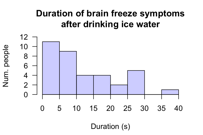
[228] recorded the length of ’brain freezes’ after consuming cold food or drink. A histogram of the data (Figure 11.17), shows \(11\) people experience symptoms less than \(5\) in length; nine people experienced symptoms for at least \(5\) but less than \(10\text{;}\) and \(1\) person experienced symptoms for at least \(35\) but under \(40\text{.}\)
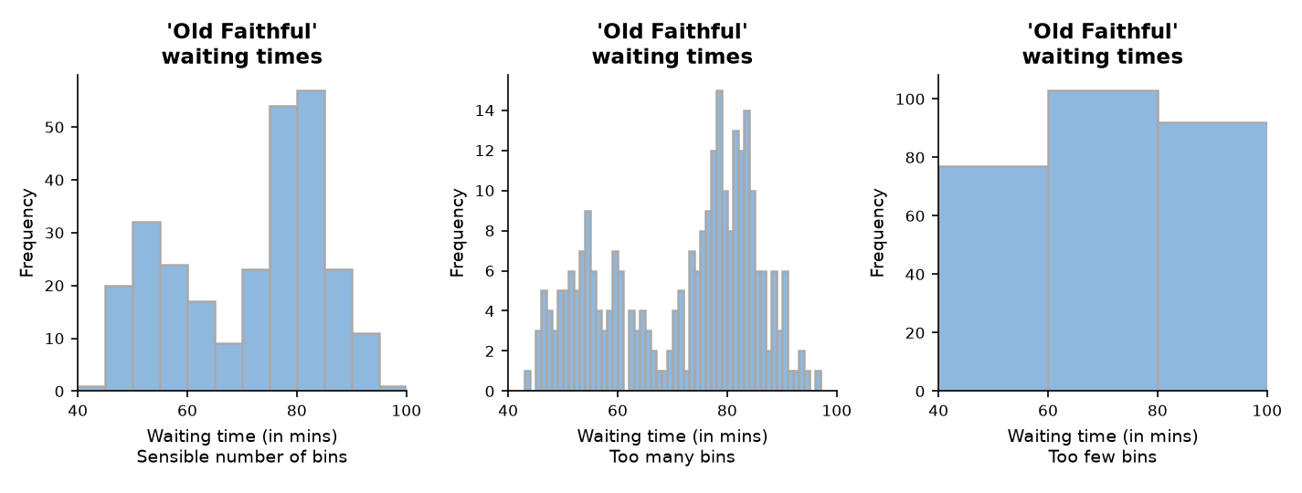
Software tries to use sensible default choices for the number of bins, and width of the bins. However, the bin size can substantially change the appearance of the histogram. Software makes it easy to try different bin sizes to find one that displays the overall distribution well.
A histogram for the time between eruptions [95] of the Old Faithful geyser in Yellowstone National Park (USA) is shown in Figure 11.19. Changing the number of bins changes the impression of the distribution.
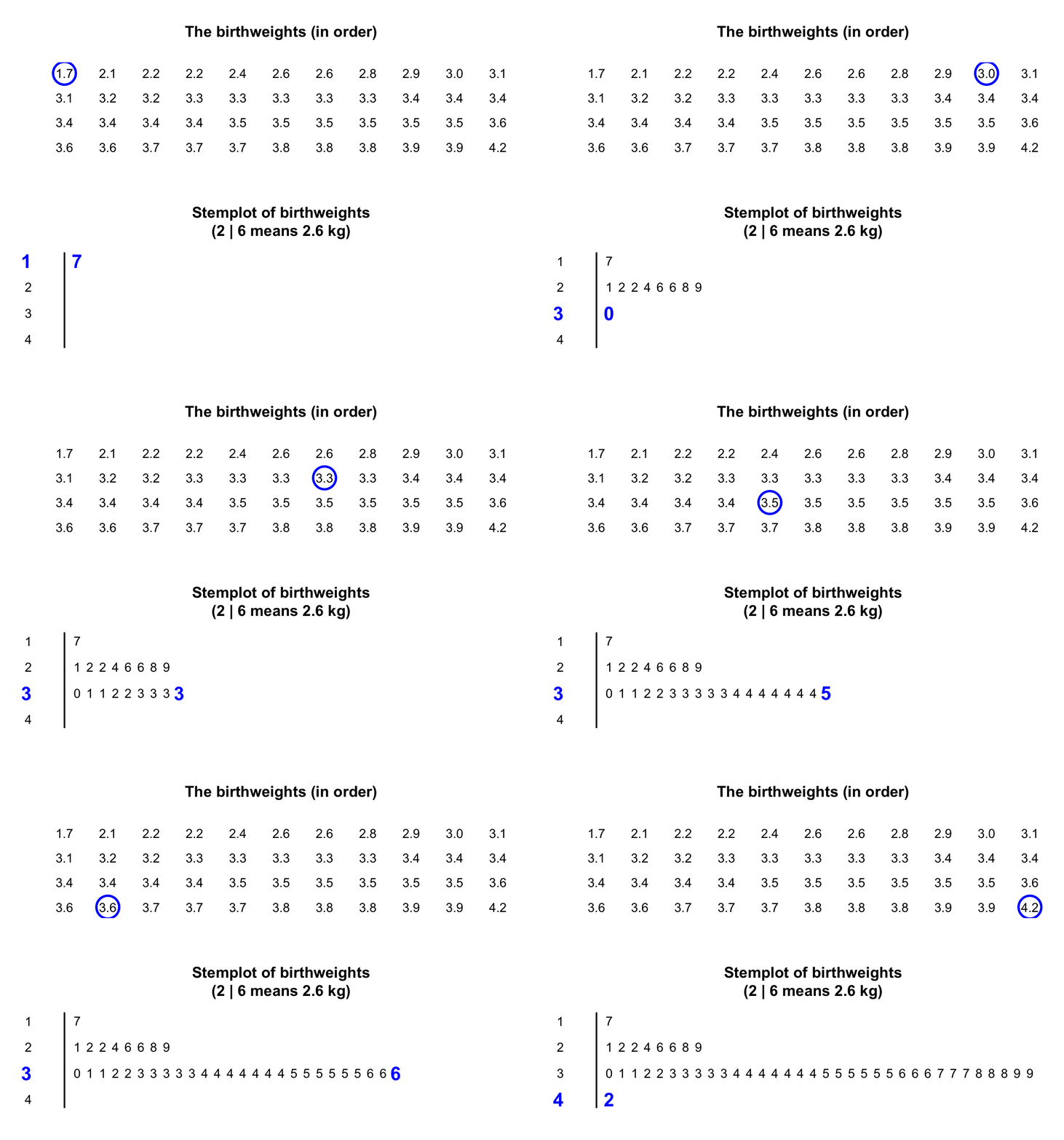
In a stemplot, part of each number is placed to the left of a vertical line (the stems), and the rest of each number to the right of the line (the leaves). The weights in Table 11.7 are given to one decimal place of a kilogram, so the whole number of kilograms is placed to the left of the line (as the stem), and the first decimal place is placed on the right of the line (as a leaf). and the first decimal place is placed on the right of the line (as a leaf). The animation below shows how the stemplot is constructed. The first weight, of \(1.7kg\text{,}\) is entered with the \(1\) to the left of the line, and the \(7\) to the right: 1 | 7. Similarly, \(2.1kg\) is entered as 2 | 1 and \(2.2kg\) is entered as 2 | 2, sharing the same stem as for \(2.1kg\text{.}\) The plot shows that most birthweights are \(3\)-point-something kilograms
the numbers in each row should be evenly spaced, with the numbers in the columns under each other, so the length of each stem is proportional to the number of observations.
add an explanation for reading the stemplot. For example, the stemplot for the baby-birth data says ’ ’2 | 6 means \(2.6kg\)’ (rather than, say, \(0.26kg\text{,}\) or \(2lb 6oz\)).
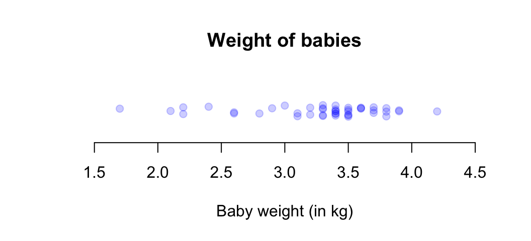
Dot charts show the data on a single (usually horizontal) axis, with each observation represented by a dot (or other symbol). Sometimes, observations are identical, or nearly so; to avoid points being plotted on top of other points (called overplotting), the points are jittered (placed with some added randomness in the vertical direction) or stacked (placed above each other).
Consider the weights (in kg) of babies born in a Brisbane hospital (Table 11.6). A dot chart (Figure 11.24) shows that most babies were born between \(3\) and \(4\text{.}\) The points have been jittered.
Graphs are constructed to help readers understand the data. Hence, after producing a graph, the distribution of the data should be described, focusing on four features:
The weights of babies (Example 11.13) are typically between about \(2.5\) and \(3\) (the average), with most between \(1.5\) and \(4.5\) (variation). A few babies have very low weights (shape), probably premature births. No unusual values are present.
The purpose of describing sample data is to understand the population that the sample comes from, and which the RQ asks about. Any computed numerical quantities (such as averages) are computed from the sample, even though the population is of interest. As a result, distinguishing parameters and statistics is important.
A statistic is a numerical value estimating an unknown population value. However, countless samples are possible (Section 6.2), and so countless possible values for the statistic—all of which are estimates of the value of the parameter—are possible. The observed value of the statistic depends on which one of the countless possible samples is selected.
The RQ identifies the population, but in practice only one of the many possible samples is studied. Statistics are estimates of parameters, and the value of the statistic is not the same for every possible sample. We only observe one value of the statistic from our single observed sample.
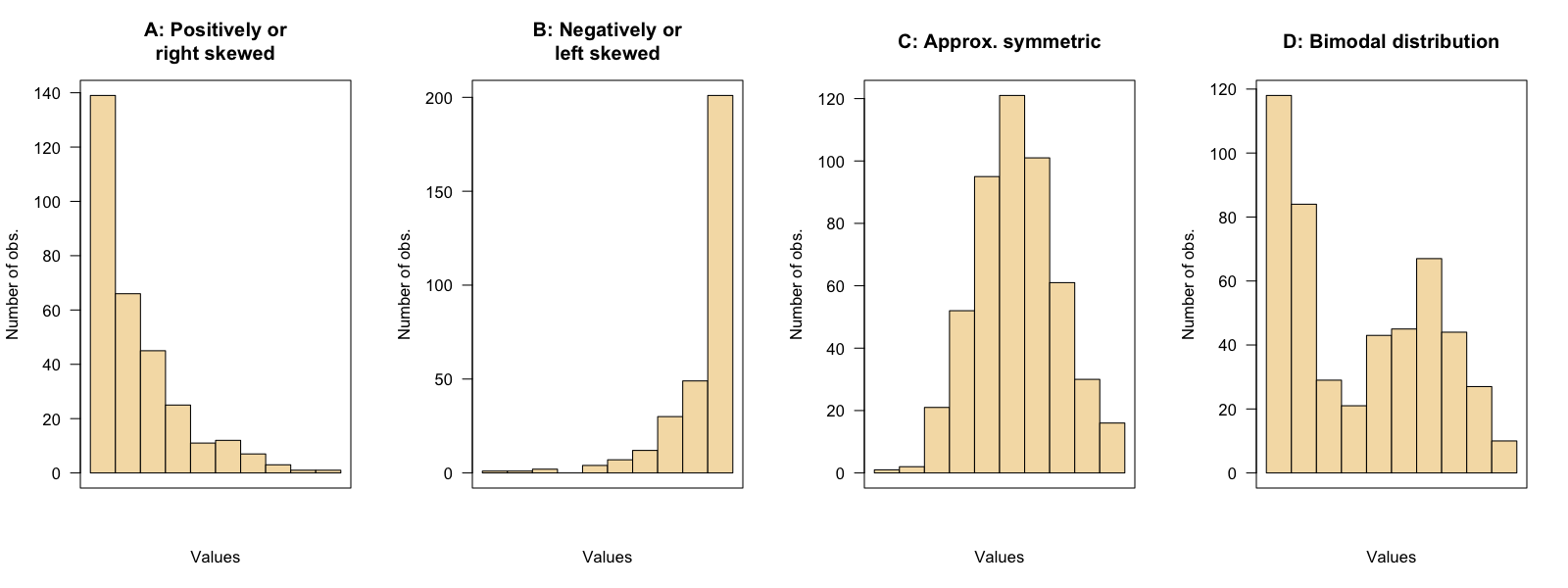
The Old Faithful geyser in Yellowstone National Park (USA) erupts regularly [95]. The histogram for the time between eruptions (Figure 11.19, left panel) is bimodal, with peaks near \(55\) and \(80\text{.}\)
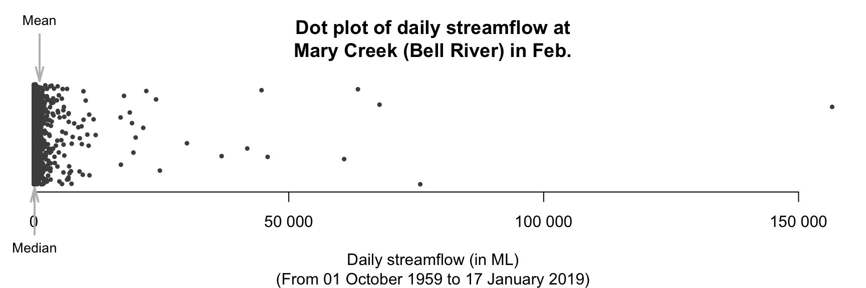
Consider the daily river flow volume (’streamflow’) at the Mary River (Queensland, Australia) from 01 October 1959 to 17 January 2019 [101]. The ’average’ daily streamflow in February could be described using either:
Both are an ’average value’, and of the same data, yet give very different values. This implies the mean and median measure the ’average’ differently, and have different meanings. Which is the best ’average’ to use? To decide, both averages need to be studied.
The mean of the population is denoted by \(\mu\text{,}\) and its value is almost always unknown. The mean of the population is estimated by the mean of the sample, denoted \(\bar{x}\text{.}\) In this context, the value of the unknown parameter is \(\mu\text{,}\) and the value of the statistic is \(\bar{x}\text{.}\)
The sample mean estimates the population mean, and every sample is likely to give a different value for the sample mean. We usually only have one sample.
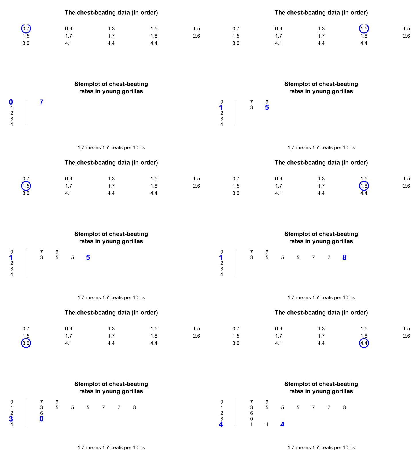
Consider a small dataset for answering this descriptive RQ: ’For gorillas aged under \(20\text{,}\) what is the average chest-beating rate?’ The population mean rate (denoted \(\mu\)) is to be estimated.
Every gorilla cannot be studied, so a sample is studied. The unknown population mean \(\mu\) is estimated using the sample mean (\(\bar{x}\)) of \(n = 14\) young gorillas (Example 11.21, top panel).
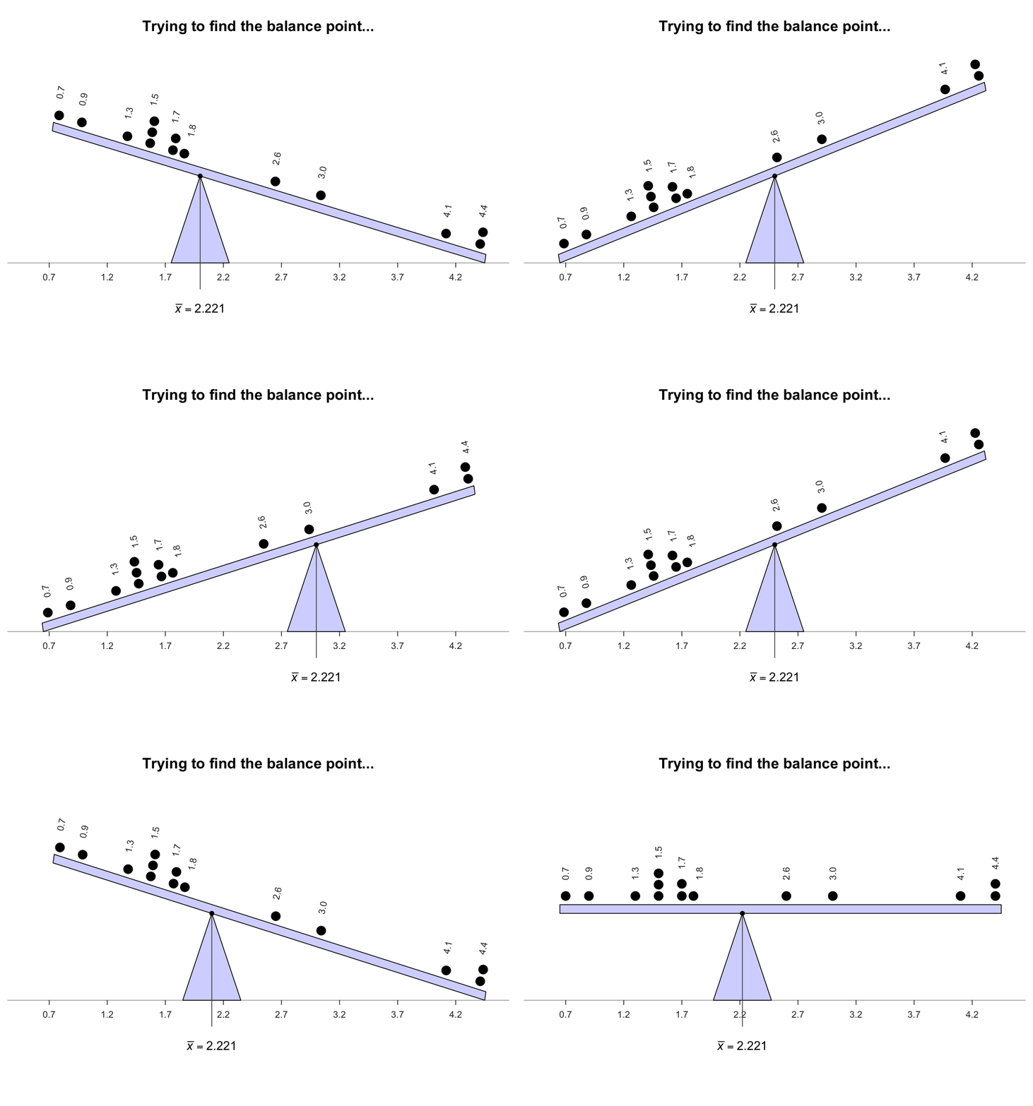
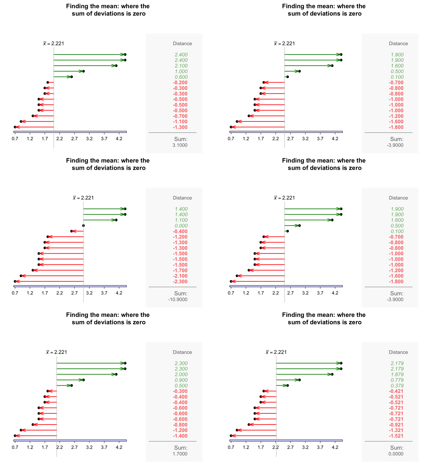
The sample mean is the ’balance point’ of the observations. The animation below shows how the mean acts as the balance point for the gorilla data. Also, the positive and negative distances (the ’deviations’) of the observations from the mean add to zero, as in the animation below. Both of these explanations seem reasonable for identifying an ’average’ value for the data.
The mean is one way to measure the ’average’ value of quantitative data. The arithmetic mean is the ’balance point’ of the data. The positive and negative distances from the mean add to zero.
To find the value of the sample mean, add (denoted by \(\sum\)) all the observations (denoted by \(x\)) then divide by the number of observations (denoted by \(n\)). In symbols:
an estimate of the population mean (i.e., the sample mean) chest-beating rate is found by summing all \(n = 14\) observations then dividing by \(n = 14\text{:}\)
The sample mean is usually calculated using statistical software for large amounts of data, or a calculator for small amounts of data. However, knowing how the mean is computed is helpful.
Software and calculators often produce numerical answers to many decimal places, not all of which may be meaningful or useful. A simple, but often useful, rule-of-thumb is to round to one or two more significant figures than the original data. Software usually does not add measurement units to the answer either.
[261] recorded the distance at which flies (Drosophila) were detected by bats for \(n = 11\) detections (Table 11.43). The population mean distance is estimated by the sample mean as \(\bar{x} = 532/11 = 48.4\) cm.
A median is a value separating the largest \(50\)% of the data from the smallest \(50\)% of the data. In a dataset with \(n\) values, the median is ordered observation number\((n + 1)/2\text{.}\) (The value of the median is not\((n + 1)/2\text{,}\) and the median not necessarily halfway between the minimum and maximum values in the data.)
Many calculators cannot find the median. The median has no commonly-used symbol, though \(\tilde{\mu}\) and \(\tilde{x}\) are sometimes used for the population and sample medians respectively.
The median is one way to measure the ’average’ value of data. A median is a value such that half the values are larger than the median, and half the values are smaller than the median.
first arrange the data in numerical order (Table 11.47). The median separates the larger seven numbers from the smaller seven numbers. With \(n = 14\) ordered observations, the median is at position \((14 + 1)/2 = 7.5\) (the median itself is not \(7.5\)). This means that the median is located between the seventh and eighth ordered observations.
Thus, the sample median, an estimate of the population median, is between \(1.7\) (ordered observation \(7\)) and \(1.7\) (ordered observation \(8\)). Since these values are the same, the sample median is \(1.7\) beats per \(10\text{.}\)
if the sample size \(n\) is even (such as the chest-beating data; Example 11.46), the median is halfway between the two middle numbers, when the observations are ordered.
The sample median estimates the population median, and every sample is likely to have a different value for the sample median. We usually only have one sample.
For the bat data (Table 11.43), the estimate of the population median distance at which bats detect the flies is the sample median. With \(n = 11\text{,}\) the median is the \((11 + 1)/2 = 6\)th ordered value, which is \(45\text{.}\)
Consider the daily streamflow at the Mary River again (Example 11.34): the sample mean daily streamflow is \(1 123\) ML, and the sample median daily streamflow is \(146.1\) ML. Which is ’best’ for measuring the average streamflow?
For these data, \(86\)% of observations are smaller than the mean, but \(50\)% of the observations are smaller than the median (by definition). The mean is hardly a central value.
A dot chart of the daily streamflow (Figure 11.51; jittered) shows that the data are very highly right-skewed, with many very large outliers (presumably flood events).
Figure11.51.A dot plot of the daily streamflow at Mary River from 1960 to 2017, for February (\(n = 1\,650\)). Many very large outliers exist. Note: values have been jittered in the vertical direction, but overplotting is still present near \(0\text{.}\)
The streamflow data are very right skewed, which is important for explaining the difference between the values of the sample mean and the sample median:
Means tend to be too large if the data contain large outliers or severe right skewness, and too small if the data contain small outliers or severe left skewness. The Mary River data contains extremely large outliers—and many of them—so the mean is much larger than the median. The median is the better measure of average for these data. However, understanding the variation is probably more important than understanding the average value (Section 11.7), and the data may even be better described using percentiles (Subsection 11.7.4).
The mean is generally used rather than the median if possible (for practical and mathematical reasons), and is the most commonly-used measure of location. However, the mean is not always appropriate (as the mean is influenced by outliers and skewness). The mean and median are similar in approximately symmetric distributions. Sometimes, quoting both the mean and the median may be appropriate.
For quantitative data, the amount of variation in the bulk of the data should be described. Many ways exist to measure the variation in a dataset, including:
As always, a value computed from a sample (the statistic) estimates the unknown value in the population (the parameter), and every sample can produce a different estimate.
The range is not often used as it only uses two values in a data set, both of which are extreme observations. As a result, the range is highly influenced by outliers. Sometimes, the range is given by stating both the maximum and the minimum value in the data instead of the difference between these values. The range is measured in the same measurement units as the data, and is usually quoted with the median.
The population standard deviation (a parameter) is denoted by \(\sigma\) and is estimated by the sample standard deviation \(s\) (a statistic). The standard deviation is the most commonly-used measure of variation. It is tedious to compute manually, so is usually calculated using statistical software for large amounts of data, or a calculator for small amounts of data.
The standard deviation is (approximately) the mean distance that observations are from the mean. This seems like a reasonable way to measure the amount of variation in data.
The sample standard deviation estimates the population standard deviation, and every sample is likely to have a different value for the sample standard deviation. We usually only have one sample.
Even though you do not have to use the formula to calculate \(s\) (use software), we will demonstrate to show exactly what \(s\) calculates. The formula for computing the value of \(s\) is
where \(\bar{x}\) is the sample mean, \(x\) represents the individual data values, \(n\) is the sample size, and the symbol ’\(\sum\)’ means to add (Subsection 11.6.1). Using the formula requires these steps.
You do not need to use the formula! You should know how to use software or a calculator to find the value of the standard deviation, what the standard deviation measures, and how and when to use it.
Example11.57.Computing a sample standard deviation.
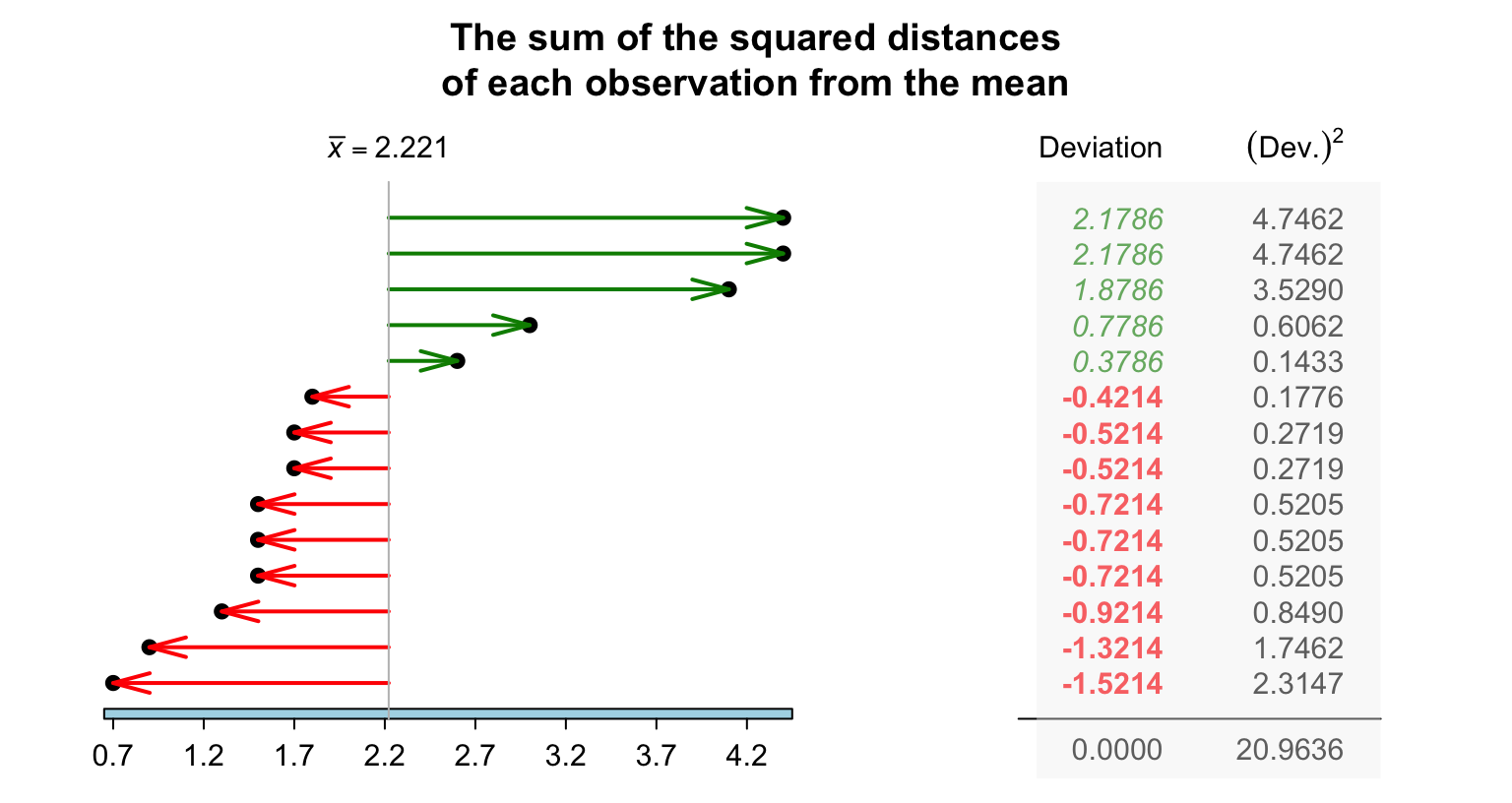
For the chest-beating data (Table 11.47), the squared deviations of each observation from the mean of \(2.2214\) (using four decimal places in calculations) are shown in Figure 11.58. The sum of the squared distances is \(20.9636\text{.}\) Then, the sample standard deviation is:
Figure11.58.The standard deviation is related to the sum of the squared-distances from the mean. The chest-beating data are used. The sum of the deviations is always zero.
Subsection11.7.3Variation: the interquartile range (IQR)
The standard deviation uses the value of \(\bar{x}\text{,}\) so is impacted by skewness and outliers just like the sample mean. A measure of variation not affected by skewness and outliers is the interquartile range, or IQR. To understand the IQR, understanding quartiles is necessary first.
The first quartile \(Q_1\) is a value separating the smallest \(25\)% of observations from the largest \(75\)%. The \(Q_1\) is like the median of the smaller half of the data, halfway between the minimum value and the median.
The third quartile \(Q_3\) is a value separating the smallest \(75\)% of observations from the largest \(25\)%. The \(Q_3\) is like the median of the larger half of the data, halfway between the median and the maximum value.
Quartiles divide the data into four parts of approximately equal numbers of observations. The interquartile range (or IQR) is the difference between \(Q_3\) and \(Q_1\text{.}\)
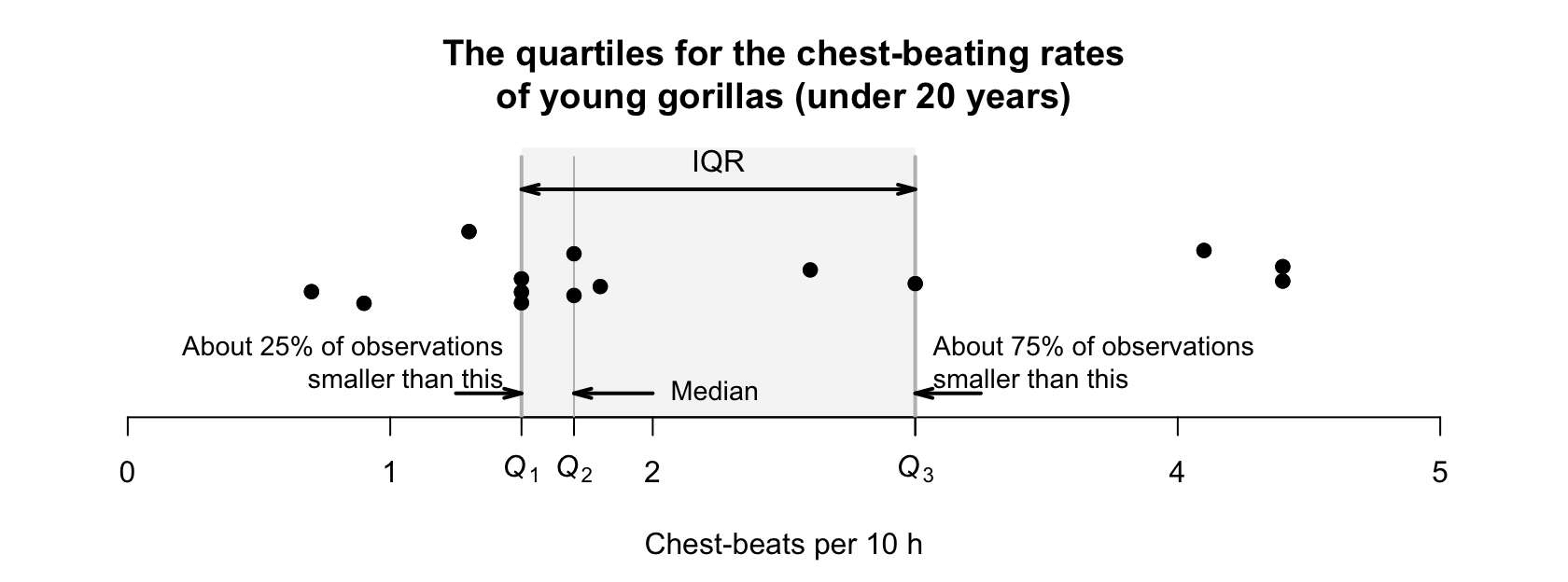
For the chest-beating data (Table 11.47), where \(n = 14\) (an even number of observations), the median is \(1.7\) (Example 11.46). The data then can be split into smaller and larger halves, each with seven values:
\(Q_1\text{,}\) the first quartile, is the median of the smaller half; \(Q_1 = 1.5\text{.}\) About \(25\)% of observations are smaller than \(1.5\text{.}\)
\(Q_3\text{,}\) the third quartile, is the median of the larger half; \(Q_3 = 3.0\text{.}\) About \(75\)% of observations are smaller than \(3.0\text{.}\)
To divide the data into four parts of equal numbers of observations, each part would need \(14/4 = 3.5\) observations, which is not possible. Hence, we say the values of \(Q_1\) and \(Q_3\) are ’about’ the values given. (Software sometimes uses a different method for computing the quartiles.) Using these values, the IQR is \(Q_3 - Q_1\) = \(3.0 - 1.5 = 1.5\text{,}\) as shown in Figure 11.62.
Since the IQR measures the range of the central \(50\)% of the data, the IQR is not influenced by outliers. The IQR is measured in the same measurements units as the data.
Software often uses different rules to compute quartiles (and medians) that may produce slightly different answers. In large datasets, the differences are usually minimal.
When \(n\) is odd, the median may or may not be included in each of these halves when computing \(Q_1\) and \(Q_3\text{;}\) we decide not to include the median in each half.
This means that the first quartile \(Q_1\) is the \(25\)th percentile, the second quartile \(Q_2\) is the \(50\)th percentile (and median), and the third quartile \(Q_3\) is the \(75\)th percentile.
Percentiles are especially useful for very skewed data in certain applications. For instance, scientists who monitor rainfall and stream heights, and engineers who use this information, are more interested in extreme weather events rather than the ’average’ event. Structures need to be designed to withstand \(1\)-in-\(100\) year events (the \(99\)th percentile) or similar, rather than ’average’ events. Percentiles are measured in the same measurements units as the data.
For the streamflow data at the Mary River (Example 11.34), the February data are highly right-skewed (Figure 11.51). The median (\(50\)th percentile) is \(146.1\) ML. However, the \(95\)th percentile is \(3 480\) ML and the \(99\)th percentile is \(19 043\) ML.
Since the standard deviation formula uses the mean, it is impacted in the same way as the mean by outliers and skewness. Hence, the standard deviation is best used with approximately symmetric data. The IQR is best used when data are skewed or outlier are present. Sometimes, both the standard deviation and the IQR can be quoted.
Outliers are ’unusual’ observations: those quite different from the bulk of the data (larger or smaller). Outliers are ’unusual’, but not necessarily ’incorrect’ or ’bad’ observations. Rules for deciding if an observation is an outlier are always arbitrary.
An outlier is an observation that is ’unusual’ (either larger or smaller) compared to the bulk of the data. Rules for identifying outliers are arbitrary.
The standard deviation rule uses the mean and the standard deviation, so is suitable for approximately symmetric distributions (when means and standard deviations are sensible numerical summaries). The rationale behind this rule is explained in Section 20.3.
All rules for identifying outliers are arbitrary, and sometimes the standard deviation rule is given slightly differently. For example, outliers may be identified as observations more than \(2.5\) standard deviations from the mean. Both rules are acceptable, since the definition is arbitrary.
Example11.70.Standard deviation rule for identifying outliers.
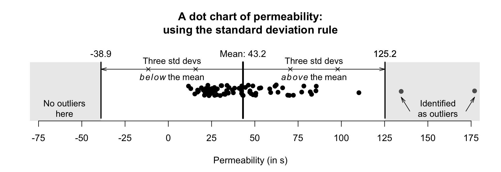
An engineering project [92] studied a new building material, to estimate the average permeability. Permeability time (the time for water to permeate the sheets) was measured from \(81\) pieces of material (in seconds).
For these data, the mean is \(\bar{x} = 43.162\) and the standard deviation is \(s = 27.358\text{.}\) Using the standard deviation rule, outliers are observations smaller than \(43.162 - (3 \times 27.358)\) or larger than \(43.162 + (3 \times 27.358)\text{;}\) that is, smaller than \(-38.9\) (which is clearly not appropriate here, as the data must be positive values), or larger than \(125.2\text{.}\) This rule is shown in Figure 11.71; two observations are identified as outliers using the standard deviation rule.
Since the standard deviation rule for identifying outliers relies on the mean and standard deviation, it is not appropriate for non-symmetric distributions. Another rule is needed for identifying outliers in these situations: the IQR rule.
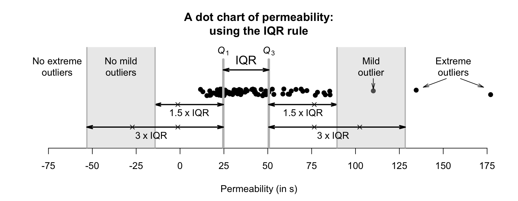
Using the permeability data seen in Example 11.70, a computer shows that \(Q_1 = 24.7\) and \(Q_3 = 50.6\text{,}\) so \(\text{IQR} = {50.6 - 24.7 = 25.9}\text{.}\) Then, extreme outliers are observations \(3 \times 25.9 = 77.7\) more unusual than \(Q_1\) or \(Q_3\text{.}\) That is, extreme outliers are observations are:
Mild outliers are observations \(1.5 \times 25.9 = 38.9\) more unusual than \(Q_1\) or \(Q_3\) (that are not extreme outliers). That is, mild outliers are
The standard deviation rule is most appropriate for approximately symmetric distributions; the IQR rule can be used for any distribution, but primarily for those skewed or with outliers.
What should be done if outliers are identified in data? Deleting or removing outliers simply because they are identified as outliers is very poor practice. After all, the outliers were obtained from the study like all other observations; they belong in the data as much as any other observation. In addition, the rules for identifying outliers are arbitrary: some observations may be identified as outliers using one rule, but not by another.
the outlier is clearly a mistake (e.g., an age of \(222\)). If the mistake cannot be fixed (e.g., the completed questionnaire form is lost), the observation can be deleted. Similarly, if the outlier comes from an error or mistake in the data collection (e.g., too much fertiliser was accidentally applied), the observation can be deleted.
the outlier represents a different population. Suppose an outlier is identified in a study of students, corresponding to a student aged 65. If the next oldest student in the data is aged \(39\text{,}\) the outlier can be removed, since it belongs to a different population (’students aged over \(40\)’) than the other observations (’students aged \(40\) and under’). The remaining observations can be analysed, but the results only apply to students aged under \(40\) (which should be clearly communicated).
the reason for the outlier is unknown. In these cases, discarding outliers routinely is not recommended; the outliers are probably real observations that are just as valid as the others. Perhaps a different analysis is necessary (e.g., using medians rather than means). Furthermore, very large datasets are expected to have a small number of observations identified as outliers using the above arbitrary rules.
The Mary River dataset (Section 11.6) has many extremely large outliers identified by software, but each is reasonable. They probably correspond to flood events (which could be confirmed). Removing these from the analysis would be inappropriate.
In studies with quantitative variables, the quantitative variables should be summarised in a table. The table should include, as a minimum, measures of average, variation and the sample sizes. An example is given in the next section (Table 11.80).
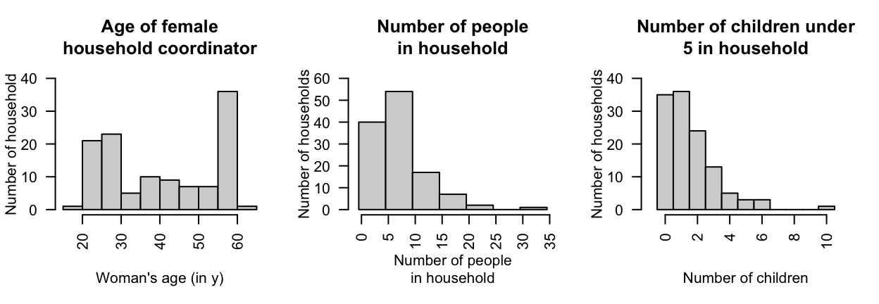
[119] recorded data about access to water for three rural communities in Cameroon. Three quantitative variables are recorded. Part of understanding the data requires summarising the quantitative variables; histograms are shown in Figure 11.79, and a summary table in Table 11.80.
Many households are coordinated by women in their late \(50\)s. The number of people and number of children under \(5\) years of age are both right-skewed. One household has over \(30\) people, and has \(10\) children in that household. (These are identified as outliers, but are unlikely to be mistakes.) Some observations are missing for some variables, explaining the differences in sample sizes in Table 11.80.
Figure11.79.The age of the female household coordinator, the number of people in the household, and the number of children in the household aged under \(5\) years, for the water-access study.
Quantitative data can be graphed using a histogram, stemplot (in special circumstances), or dot charts. Quantitative data can be summarised numerically; the most common techniques are indicated in Table 11.81. The mean and standard deviation are usually used whenever possible, for practical and mathematical reasons. Sometimes quoting both the mean and median (and the standard deviation and IQR) may be appropriate.
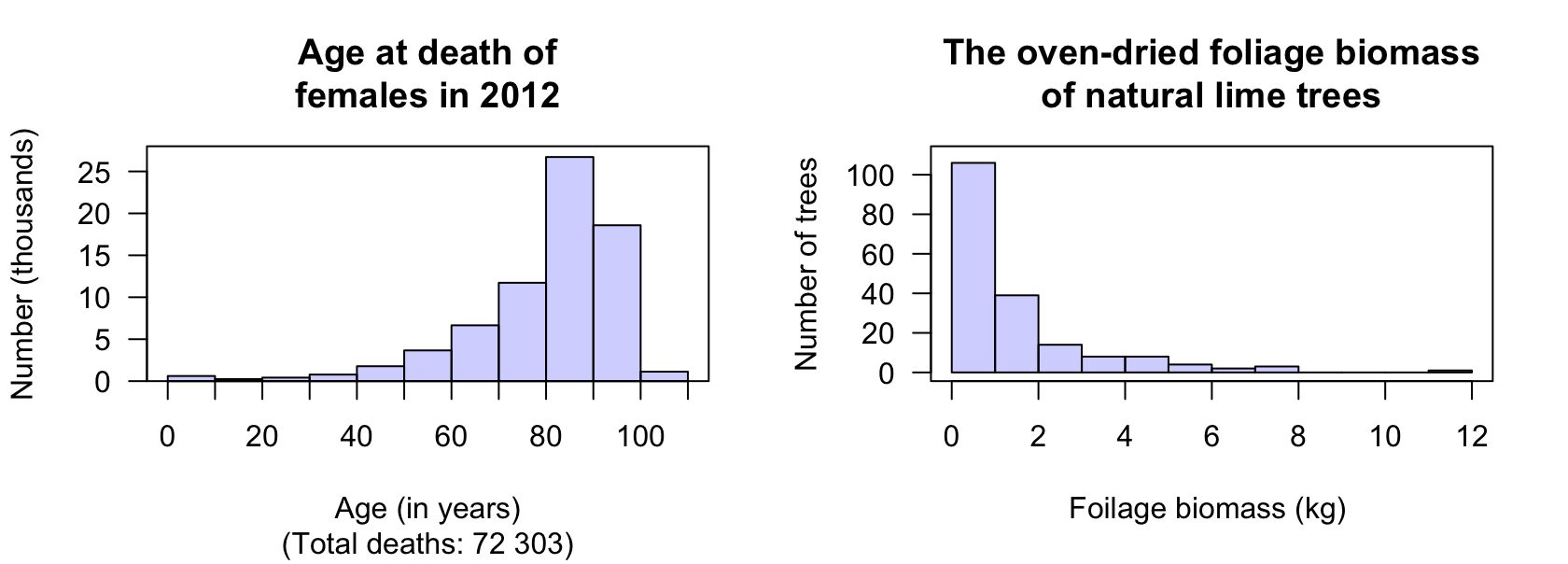
The Australian Bureau of Statistics (ABS) records the age at death of Australians. The histogram of the age of death for females in 2012 is shown in Figure 11.82 (left panel). Describe the distribution.
[Dataset: Lime] [303] measured the oven-dried foliage biomass of lime trees grown in natural environments. The histogram of the foliage biomass is shown in Figure 11.82 (right panel). Describe the distribution.
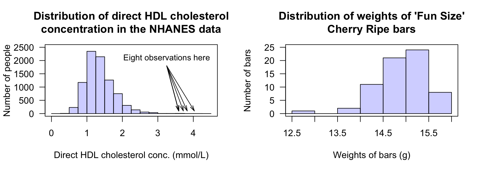
[Dataset: NHANES] The histogram of the direct HDL cholesterol concentration from the American National Health and Nutrition Examination Survey (nhanes) [130] from \(1999\)–\(2004\) is shown in Figure 11.83 (left panel).
Figure11.83.Left: the histogram of direct HDL cholesterol concentration from the nhanes study (large outliers exist but are hard to see, as the sample size is very large). Right: the weights of ’Fun Size’ Cherry Ripe chocolate bars.
[Dataset: CherryRipe] The histogram of the weights of ’Fun Size’ Cherry Ripe chocolate bars between 2016 and 2019 is shown in Figure 11.83 (right panel).
[215] studied fulmars (a seabird). The mass of the female birds were (in grams): \(635\text{;}\)\(635\text{;}\)\(668\text{;}\)\(640\text{;}\)\(645\text{;}\)\(635\text{.}\)
Draw a stemplot of the average monthly SOI (from the Australian Bureau of Meteorology) in August from \(1995\) to \(2003\) (Table 11.85). Then, use your calculator (where possible) to calculate the:
[Dataset: Orthoses] [309] studied the influence of using ankle-foot orthoses in children with cerebral palsy. The data for the \(15\) subjects is shown in Table 10.24.
An article studied patients who had been admitted to Castle Hill Hospital [211]. The total number of microplastics found in the lungs of each patient are shown in Table 11.87. For these patients:
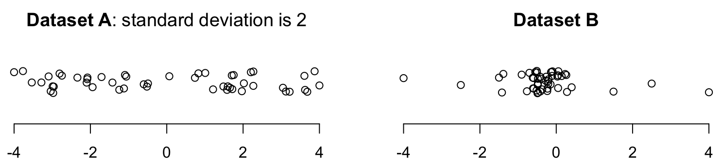
The standard deviation for Dataset A in Figure 11.88 is \(s = 2\text{.}\) Will the standard deviation of Dataset B be smaller than or greater than \(2\text{?}\) Why?
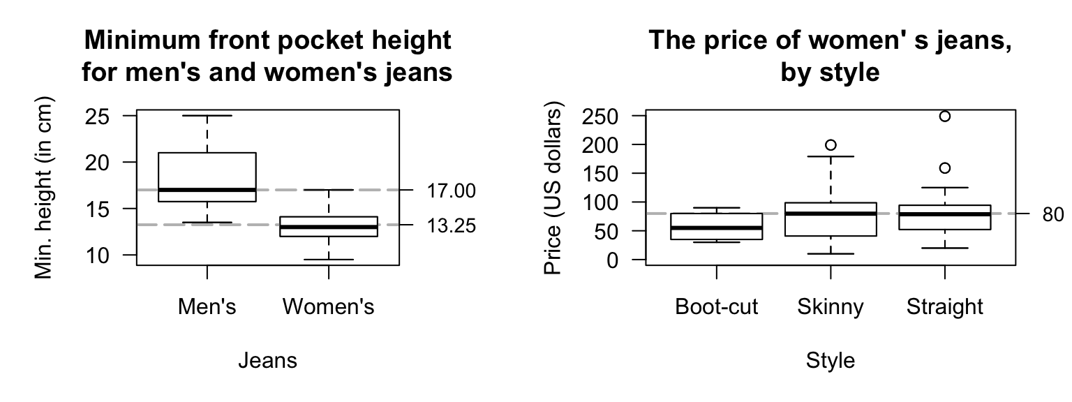
[Dataset: Jeans] [297] recorded the size of pockets in men’s and women’s jeans, including the minimum heights of the front pockets (Figure 11.89, left panel).
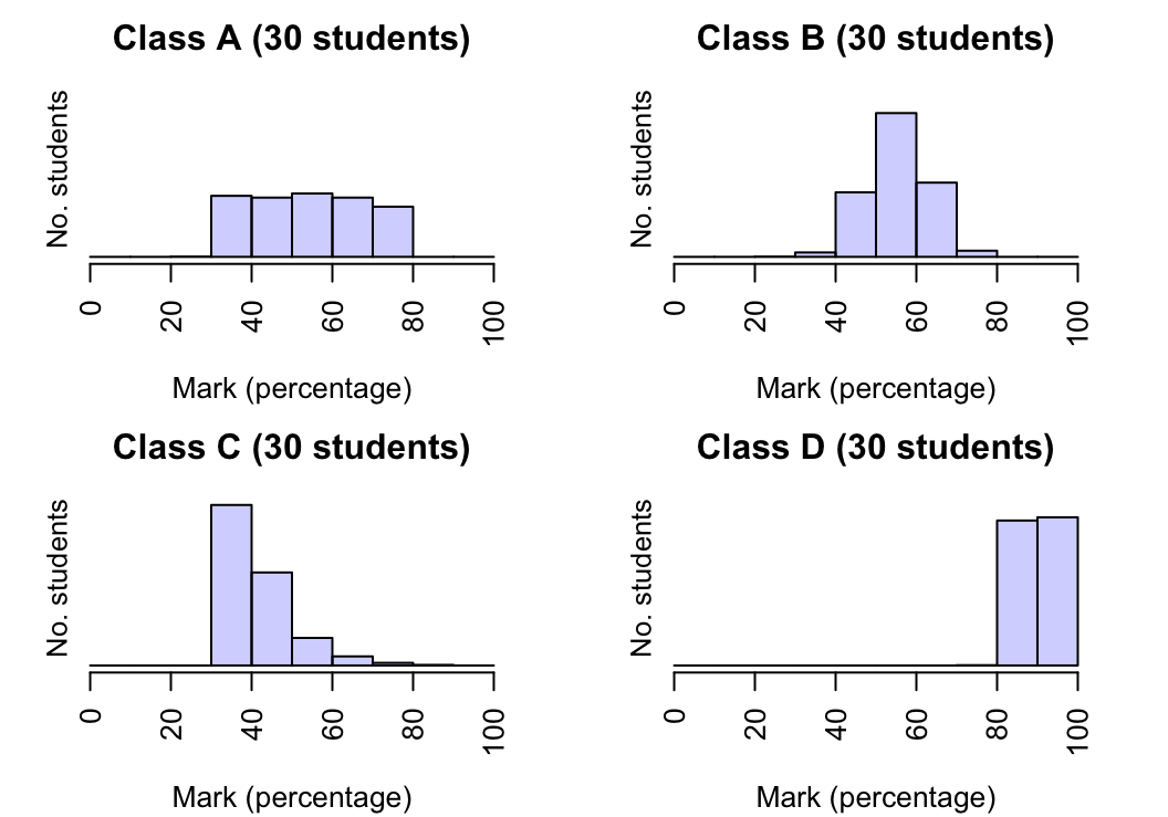
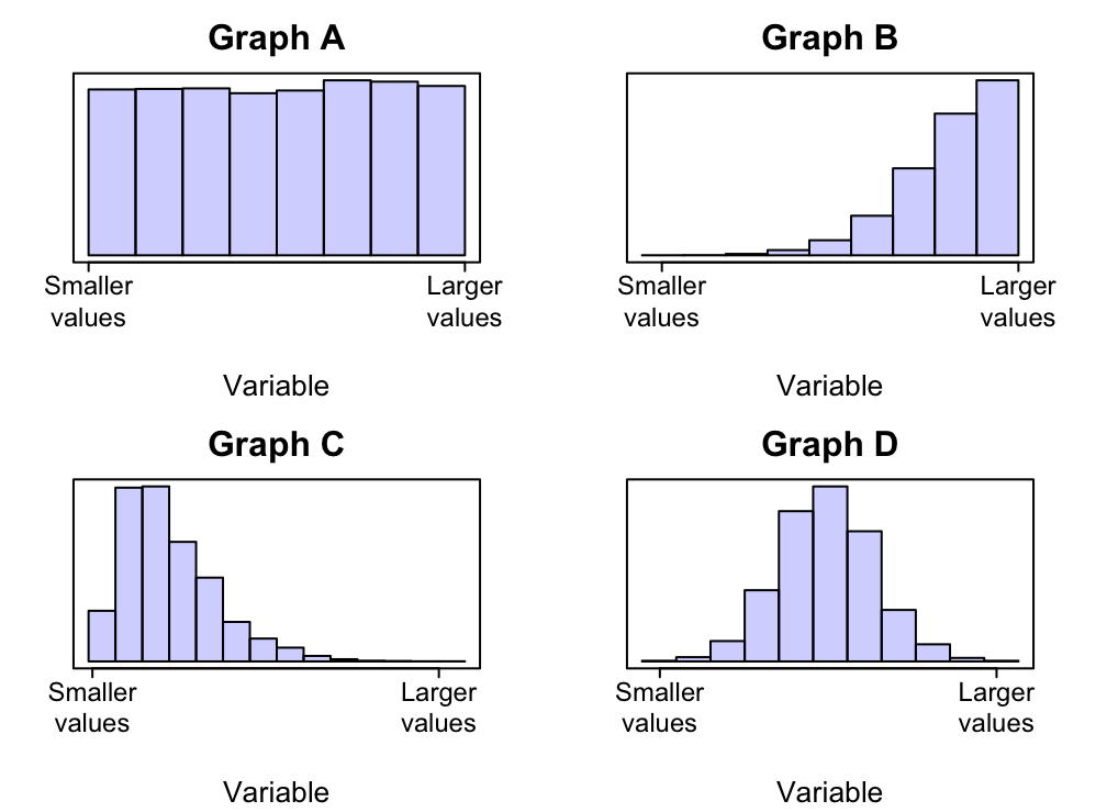
A professor has recorded the marks (as a percentage) for all students in her four classes for an assignment. All classes have the same number of students. The corresponding histograms are shown in Figure 11.90.
(The first bar of the histogram is not necessarily at zero; it is the shape of the histogram that is of interest here: right skewed, left skewed, symmetric, etc.)