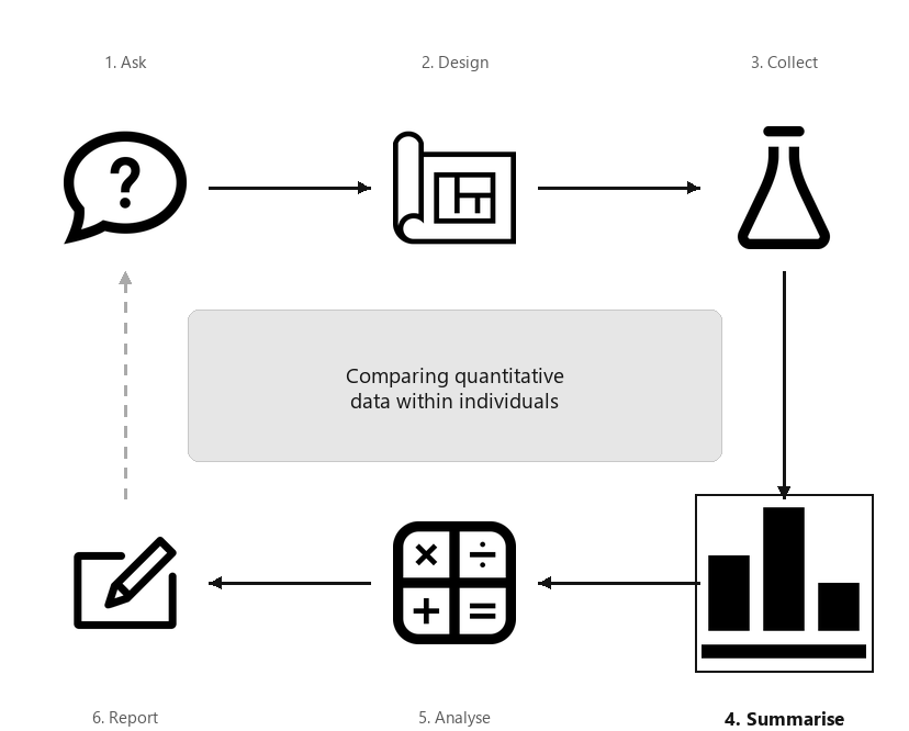
A diagram showing the six steps of research, arranged in a cycle: Ask, Design, Collect, Classify and summarise, Analyse, Report. Step 4 (Summarise) is highlighted, captioned “Comparing quantitative data within individuals”.
Sometimes the same quantitative variable is measured on each individual more than once (i.e., within-individual changes for each unit of analysis) but only a small number of times. Examples of this type of data include:
In both cases, the same variable is measured multiple times for each individual. This chapter studies summarising within-individuals changes in quantitative variables.
When each individual has two observations, the difference between the observations can be computed for each individual. Then, the appropriate numerical summary is to summarise these differences over all individuals; for example, using the mean of these differences.
When more than two observations are made for each individual, the changes from the first observation (the reference level) may be computed (e.g., if the first observation is pre-intervention, or a benchmark, observation); for example, using the mean change (see Sect. Section 13.5).
[111] studied children with atopic asthma, and measured the immunogoblin E concentrations (IgE) before and after an intervention for each child (Table Table 13.2), plus the reduction in IgE for each child. The child is the individual.
In the numerical summary table, the information for the differences is not found by subtracting the information in one row from the other. In Table Table 13.3, for example, the number of differences is not \(11 - 11 = 0\text{;}\) the standard deviation of the differences is not\(1615.53 - 1354.28 = 261.25\,\mu\text{g}\,\text{L}^{-1}\text{.}\) These statistics are computed from the differences (i.e., the Reductions in Table Table 13.2).
Sometimes the same variable is measured on each unit of analysis twice, when the changes (or differences) for each individual can be produced, and a histogram of the changes or differences can be constructed. The direction of the differences should be clear (e.g., first measurement minus second, or second measurement minus first).
The axis displaying the counts (or percentages) should start from zero, since the height of the bars visually implies the frequency of those differences (see Example Example 17.5).
Sometimes the variable is measured or recorded more than twice, and so a single set of differences cannot be produced. In these cases, the values for each individual can be plotted using a case-profile plot: the measurements are shown on one axis (usually the vertical), and the various points at which measurements are taken are shown on the other axis. A case-profile plot is still useful for paired data, of course.
The axis displaying the counts (or percentages) need not start from zero, since the distance from the axis to the lines do not visually imply any quantity of interest. Rather, the relative changes represented by the lines display the quantity of interest.
For the IgE data (Table Table 13.2), the measurements of IgE for each child at both times can be shown in a case-profile plot (Fig. Figure 13.9, right panel).
Figure13.9.The IgE data. Left: a histogram of the differences (reductions); boundary observations are counted in the lower box. Right: a case-profile plot, where each line joins each person’s pre-intervention to their post-intervention measurement.
Runners use wearable devices to measure many performance indicators, including vertical oscillation (VO). VO contributes to running economy and injury risk, so reliable VO measurements are crucial. [105] compared four devices, and obtained data from video analysis for \(n = 150\) athletes; that is, each participant had the same runs measured using five methods. The case-profile plot (Fig. Figure 13.23) shows the means for each method using a solid point; each line represents one runner. NOVA and Footpod give smaller VO measurements in general.
As in Example Example 13.10, the case-profile plot is hard to read with large numbers of individuals, and so sometimes the mean (or median, as appropriate) is shown, with some measure of the variation of the observations (Fig. Figure 13.23 shows the minimum and maximum values for each method, for instance).
Skypilot (Polemonium viscosum) is a native alpine wildflower growing in the Colorado Rocky Mountains (USA). In recent years, a willow shrub (Salix) has been encroaching on skypilot territory and, because willow often flowers early, researchers [117] are concerned that the willow may ’negatively affect pollination regimes of resident alpine wildflower species’ (p. \(6\,965\)). One RQ was:
The site is the individual; the data are paired (Sect. Section 29.1), a form of blocking (Sect. Section 7.2). The ’first-flowering day’ is the number of days since the start of the year (e.g., January 12 is ’day 12’) when flowers were first observed.
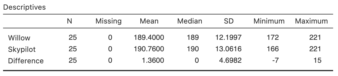
Since the data are available, the data should be summarised graphically (Fig. Figure 13.14) and numerically (Table Table 13.13), using software output (Fig. Figure 13.12).
Figure13.14.The flowering-day data. Left: a histogram of the difference between the first-flowering days (skypilot minus willow). Right: a case-profile plot of days of first flowering (unfilled points and dashed lines indicate earlier or same dates for willow).
[118] studied the effect of using Kinesio Tape to alleviate pain in athletes. Pain was measured by applying a slow constant rate of pressure on the left arm, and subjects pressed a button when the sensation moved from pressure to pain. The pressure at which this occurred was recorded. This was repeated \(5\) minutes before applying the tape, \(5\) minutes after applying the tape, and again \(15\)–\(20\) minutes after applying the tape.
Figure Figure 13.15 shows the reported pain for \(16\) subjects. A summary table is shown in Table Table 13.16. The pain thresholds are increasing slightly as time progresses.
Figure13.15.Pain threshold (left arm) at three time points when using Kinesio Tape, without applying tension, for \(n = 16\) subjects. The filled, black points represent the means for each time point.
Quantitative data measured within individuals can be summarised using a histogram of differences when the variable is measured or observed twice, or a case-profile plot (with two or more measurement or observations per individual). A summary table should show the numerical summaries for the quantitative variable at each measurement or observation and for appropriate changes.
[Dataset: Insulation] The Electricity Council in Bristol wanted to determine if a certain type of wall-cavity insulation reduced average energy consumption in winter [112][113]:
[Dataset: Captopril] In a study of hypertension [113][114], \(15\) patients were given a drug (Captopril) and their systolic blood pressure measured (in mm Hg) immediately before and two hours after being given the drug (Table Table 13.18).
[Dataset: PainRelief] [110] measured the reported pain of new mothers in Dodoma (Tanzania) at four times: near giving birth, then \(20\text{,}\)\(40\) and \(60\) minutes after giving birth. Mothers were administered either paracetamol or a cold pack as pain relief. Pain was recorded using a ’numeric rating scale represented by the horizontal line marked from zero to ten’, where higher scores mean greater pain.
Since the number of individuals is large (\(n = 912\)), use the summary data in Table Table 13.19 to sketch a plot of the means and the range, like that in Figure Figure 13.15.
[Dataset: Stress] The concentration of beta-endorphins in the blood is a sign of stress. One study ([113], Dataset 232; [116]) measured the beta-endorphin concentration for \(19\) patients about to undergo surgery.
Each patient had their beta-endorphin concentrations measured \(12\)–\(14\) hours before surgery, and also \(10\) minutes before surgery. A numerical summary (from software output) is in Table Table 13.20.
[Dataset: WCTennis] [108] recorded the push-time for French wheelchair tennis players, while holding and not holding a racquet (Table Table 13.21; [109]).
Figure13.23.Vertical oscillation (VO) measured using five methods for \(150\) runners. The solid black points represent the means for each method. Left: a line is plotted for each individual. Right: only the means are shown, with vertical lines from the minimum value to the maximum value for each method.