A diagram showing the six steps of research, arranged in a cycle: Ask, Design, Collect, Classify and summarise, Analyse, Report. Step 4 (Summarise) is highlighted, captioned “Comparing qualitative data between individuals”.
Relational RQs compare groups. This chapter considers how to compare qualitative variables in different groups. Graphs are useful for this purpose, and a table including odds, odds ratios and proportions is usually produced also.
When more than one qualitative variable is recorded for each individual, the data can be collated into a table. When two qualitative variables are cross-tabulated, the resulting table is called a two-way table. The categories for each variable should be exhaustive (cover all levels) and mutually exclusive (observations belong to one and only one level). Usually, the levels of the explanatory variable are in the rows of the table.
Both variables are qualitative with two levels, and each treatment was used on \(350\) patients. Treatment A was used from 1972–1980, and Treatment B from 1980–1985; that is, treatments were not randomly allocated, and so confounding may be present. For this reason, the researchers also recorded the size of the kidney stone (‘small’ or ‘large’) as one possible confounding variable. Firstly, consider just the small stones[97], displayed in the two-way table in Table Table 15.2.
Each variable in a two-way table can be analysed separately, using percentages or proportions (Sect. Section 12.4) or odds (Sect. Section 12.5). For example, the two variables in Table Table 15.2 (Method; Result) can be analysed separately. For overall results:
the odds that a procedure was successful is \(315/42 = 7.5\text{;}\) that is, there were \(7.5\) times as many successful procedures as unsuccessful procedures.
The data in Table Table 15.2 can be summarised by computing proportions or percentages by row. Each row refers to a different method, so row percentages will compute success percentages for the two methods.
For the small kidney stones (Table Table 15.2), the row percentages (Table Table 15.4) give the percentage of successes for each Method, since the rows represent the counts for Methods A and B. Row proportions (or percentages) allow the proportions (or percentages) within the rows (i.e., for each Method) to be compared:
For small kidney stones, Method A is slightly more successful (\(93.1\)%) than Method B (\(86.7\)%) in the sample. These percentages are collated in Table Table 15.4.
For the small kidney stones (Table Table 15.2), the column percentages (Table Table 15.6) give the percentage of successes within each column (i.e., for successes and for failures), since the columns contain the procedure results. Column percentages (or proportions) allow the percentages (or proportions) within columns to be compared:
the odds of a success coming from Method A is \(81/234 = 0.346\text{;}\) there are \(0.346\) times as many Method A procedures than Method B procedures among the successes.
the odds of failure coming from Method A is \(6/36 = 0.167\text{;}\) there are \(0.167\) times as many Method A procedures than Method B procedures among the failures.
Comparing rows (i.e., using row percentages and row odds) seems more intuitive than column proportions here: they compare the success percentages and odds for each method.
The data can be graphed by using a bar for each level of one variable, and stacking the bars for the levels of the second variable. Bars indicate the counts (or percentages) in each category. The levels can be on the horizontal or vertical axis, but placing the level names on the vertical axis often makes for easier reading, and room for long labels.
The axis displaying the counts (or percentages) should start from zero, since the height of the bars visually implies the frequency of those observations (see Example Example 17.5).
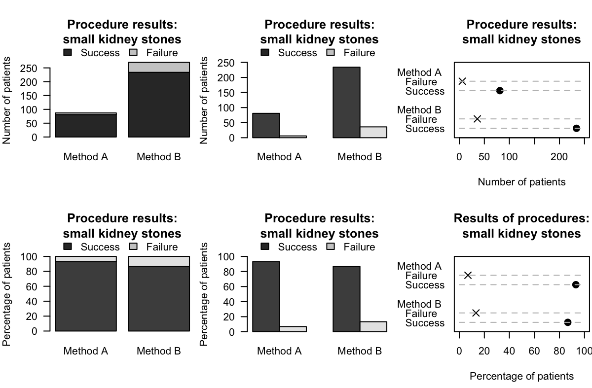
For the small kidney-stone data in Example Example 15.1, a stacked bar chart can be created by producing a bar for each method, and stacking the successes and failures for each method (Fig. Figure 15.13, top left panel).
Rather than using numbers, the percentages separately within each group can be used too (Fig. Figure 15.13, bottom left panel). This makes comparing the relative proportions easier.
Instead of stacking the success and failures bars on top of each other, these bars can be placed side-by-side for each method. Bars indicate the counts (or percentages) in each category. The levels can be on the horizontal or vertical axis, but placing the level names on the vertical axis often makes for easier reading, and room for long labels.
The axis displaying the counts (or percentages) should start from zero, since the height of the bars visually implies the frequency of those observations (see Example Example 17.5).
For the small kidney-stone data in Example Example 15.1, a side-by-side bar chart can be created by producing two bars for each method (one for failures; one for successes), and placing these side-by-side (Fig. Figure 15.13, centre panels). Again, numbers or percentages within each method can be graphed.
The axis displaying the counts (or percentages) should start from zero, since the distance of the dots from the axis visually implies the frequency of those observations (see Example Example 17.5).
For the data in Example Example 15.1, a dot chart can be created by placing plotting symbols for each result (one for failures; one for successes) side-by-side for each method (Fig. Figure 15.13, right panels). Again, numbers or percentages can be used.
using percentages or counts on one axis. (The percentages can be percentages of the total, or within the total for each level of the variable, as in the bottom plots in Fig. Figure 15.13.)
The guiding principle remains: the purpose of a graph is to display the information in the clearest, simplest possible way, to facilitate understanding the message(s) in the data.
Using a computer to create graphs is recommended, and using a computer makes it easy to try different variations to find the graph that best displays the message in the data.
Figure15.13.Six plots for the small kidney-stone data. Top plots: displaying the numbers for each method. Bottom plots: displaying the percentages for each method. Left: stacked bar chart. Centre: side-by-side bar charts. Right: dot charts.
Section15.5Numerical summary: difference between proportions
The difference between the success-rates of the two methods for the small kidney-stone data (Table Table 15.2) can be summarised using the difference between the respective proportions:
The difference between these proportions is \(\hat{p}_A - \hat{p}_B = 0.064\) (i.e., the success rate is higher for Method A). The difference between the proportions is a statistic, and the (unknown) difference between the population proportions (i.e., \(p_A - p_B\)) is a parameter.
The odds of success for Method A and Method B are very different. In the sample, the odds of success for Method A is many times greater than for Method B. In fact, in the sample, the odds of success for Method A is \(13.5\div 6.5 = 2.08\)times the odds of a success for Method B. This value is the odds ratio (OR). The sample OR is a statistic, and the (unknown) population OR is a parameter. There is no commonly-used symbol for odds ratios.
The odds ratio (often written OR) is the ratio of the odds of a result of interest in one group, compared to the odds of the same result in a different group:
For the small kidney-stone data, the odds of a success for Method A is \(81\div6 = 13.5\text{.}\) The odds of a success for Method B is \(234\div 36 = 6.5\text{.}\) The OR is then computed as \(13.5\div 6.5 = 2.08\text{.}\) The odds have been computed with the rows.
Most software computes the OR from a two-way table by using the values in the first row and first column on the top of the fractions when computing the odds and the odds ratio. In Example Example 15.15, for instance, the odds for both methods were computed with the Column 1 values on the top of the fraction (\(81\) and \(234\)), and the OR comparing the rows was computed with the Row 1 odds (\(13.5\)) on top of the fraction.
the odds in each column compares Row 1 counts (top) to Row 2 counts (bottom). The OR then compares the Column 1 odds (top) to the Column 2 odds (bottom).
Odds and ORs are computed with the first row and first column values on the top of the fraction. While both are correct, the levels of the explanatory variable are usually the rows of the table (as in Table Table 15.2), so usually the second interpretation makes more sense (as in Example Example 15.15).
The OR compares the odds of the same result (e.g., success) in two groups (e.g., Method A and Method B). This means a \(2\times 2\) table can be summarised with one number: the OR.
The numerical summary information for comparing qualitative variables can be collated in a table. The data should be summarised by one of the qualitative variables, producing proportions (or percentages) and odds for the other. The summary table also requires the differences between the proportions (or percentages) and the odds ratio.
The data in Table Table 15.2 are for procedures on small kidney stones. Data were also recorded for the large kidney stones (Table Table 15.19). As for small kidney stones, the success proportions can be computed for both methods:
So, could the data for small (Table Table 15.2) and large kidney stones (Table Table 15.19) be combined, to produce a single two-way table of just Method and Result (Table Table 15.20)?
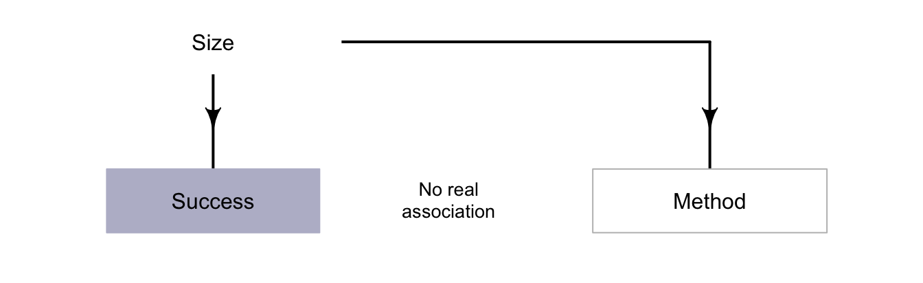
That seems strange: Method A performs better for small and for large kidney stones, but Method B performs better when combining all kidney stones. The explanation is that the size of the stone is a confounding variable (Fig. Figure 15.21). Size is associated with both the method (small stones are treated more often with Method B) and with the result (small stones have a higher success proportion for both methods). Method B was used more often on smaller kidney stones, for which a success is more likely (due to their smaller size).
This confounding could have been avoided by randomly allocating a treatment method to patients. However, random allocation was not possible in this observational study, so the researchers used a different method to manage confounding: recording the size of the kidney stones to use in the analysis (see Sect. Section 7.2).
In this example, incorporating information about a potential confounder (the size of the kidney stone) is important, otherwise the wrong (opposite) conclusion is reached: Method B would be incorrectly considered better if the size of the stones was ignored, when the better method really is Method A.
This is called Simpson’s paradox. If the size of the kidney stone had not been recorded, size would be a lurking variable, and the incorrect conclusion would have been reached.
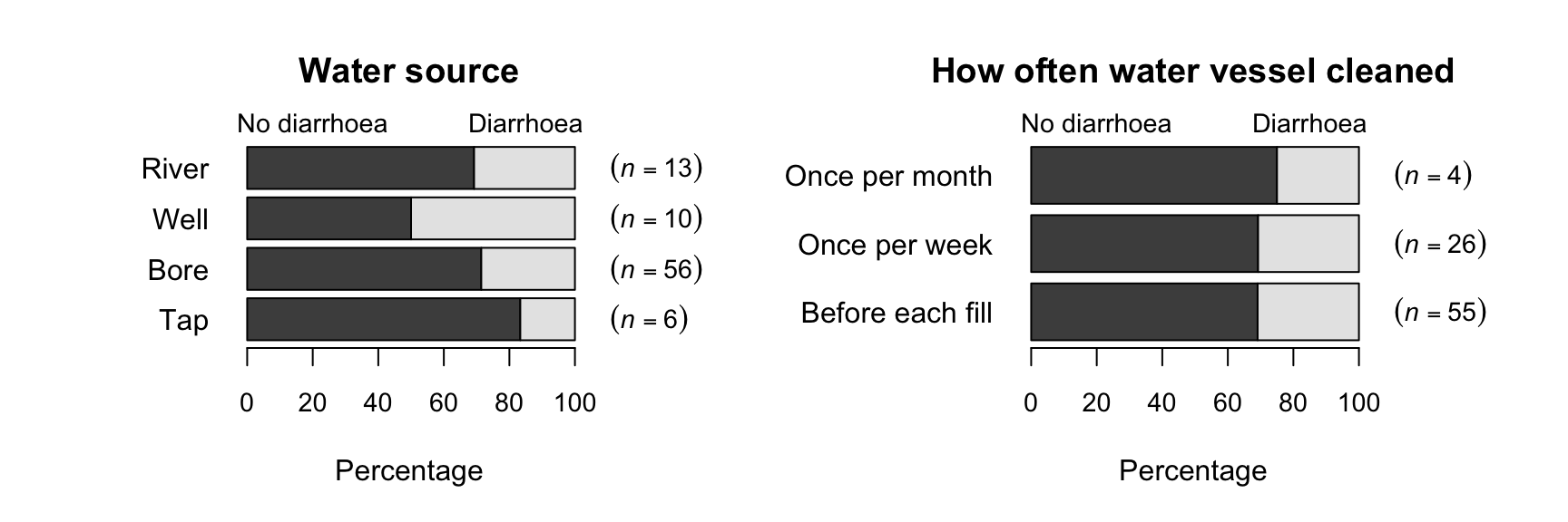
[119] recorded data about access to water for three rural communities in Cameroon (see Sects. Section 11.10 and Section 12.8). The study could be used to determine associations to the incidence of diarrhoea in young children (\(85\) households had children under \(5\)). A cross-tabulation (Table Table 15.22) shows the relationship with keeping livestock; the numerical summary table (Table Table 15.23) may suggest a difference in the percentage of children with diarrhoea in households that do and do not keep livestock. The comparison in Fig. Figure 15.24 includes some categories with small sample sizes, so the percentages shown may not be precise estimates of the population values.
As usual, the data come from one of countless possible samples, but the RQ is about the population, so making a definitive decision about the population is difficult.
Table15.22.Cross-tabulation of having livestock in the household, and children under \(5\) years of age having diarrhoea in the household in the last two weeks.
Table15.23.Numerical summary of the water-access data: odds and percentage of children with diarrhoea in the last two weeks (comparing those without livestock to those with).
Figure15.24.Percentage of children with and without diarrhoea in the last two weeks, by water source (left) and how often the water vessel was cleaned (right).
Qualitative data can be compared between different groups (between-individuals comparisons) using a stacked bar chart, side-by-side bar chart or a dot chart. The data can be displayed in a two-way table, then summarised numerically by comparing proportions (or percentages) and odds. The odds ratio (OR) and the difference between the proportions (or percentages) can be used to compare the two different groups.
[135] examined social media use (Table Table 15.25), using a representative sample of Queenslanders at least \(18\) years of age (from the \(2013\)Queensland Social Survey).
Suppose the sample OR (Row 1 divided by Row 2) has a value smaller than one. Will the difference between the sample proportions (Row 1 minus Row 2) be a positive or a negative value? Explain carefully.
[136] studied hangovers and recorded, among other information, when people vomited after consuming alcohol. Table Table 15.26 shows how many people vomited after consuming beer followed by wine, and how many people vomited after consuming only wine.
[137] recorded the sex of adult and young wallabies at the East Point Reserve, Darwin. In December 1993, \(91\) males and \(188\) female adult wallabies were recorded, and \(13\) male and \(22\) female young wallabies were recorded.
[Dataset: EmeraldAug] The Southern Oscillation Index (SOI) is a standardised measure of the air pressure difference between Tahiti and Darwin, shown to be related to rainfall in some parts of the world [134], and especially Queensland, Australia [133][142].
The rainfall at Emerald (Queensland) was recorded for Augusts between 1889 and 2002 inclusive [143], for months when the monthly average SOI was positive and non-positive (zero or negative); see Table Table 15.27.
Soccer is a unique in that one aspect is ‘the purposeful use of the unprotected head for controlling and advancing the ball’ [141]. Some researchers suspect that repeatedly ‘heading’ the ball may impair brain function. [141] studied (p. 157)
the student type, where each student was classified as a ‘soccer player’ (\(63\) students), a ‘non-soccer athlete’ (\(96\) students), or a ‘non-athlete’ (\(81\) students).
the number of head concussions, where each student was asked about the number of head concussions they had experienced; ‘zero’ (\(158\) students), ‘one’ (\(45\) students), or ‘two or more’ (\(37\) students) concussions.
Compute the OR comparing the odds of a non-athlete player receiving two or more concussions to the odds of a soccer player receiving two or more concussions.
[Dataset: PremierL] In the 2019/2020 Premier League season, Chelsea had \(4\) wins from \(10\) games at home, and \(7\) wins from \(11\) wins away from home. What is the OR of a win (comparing home games and away games)?