Chapter14Comparing quantitative data between individuals
Objectives
So far, you have learnt to ask an RQ, design a study, collect the data, and describe the data. In this chapter, you will learn to compare quantitative data in different groups. You will learn to:
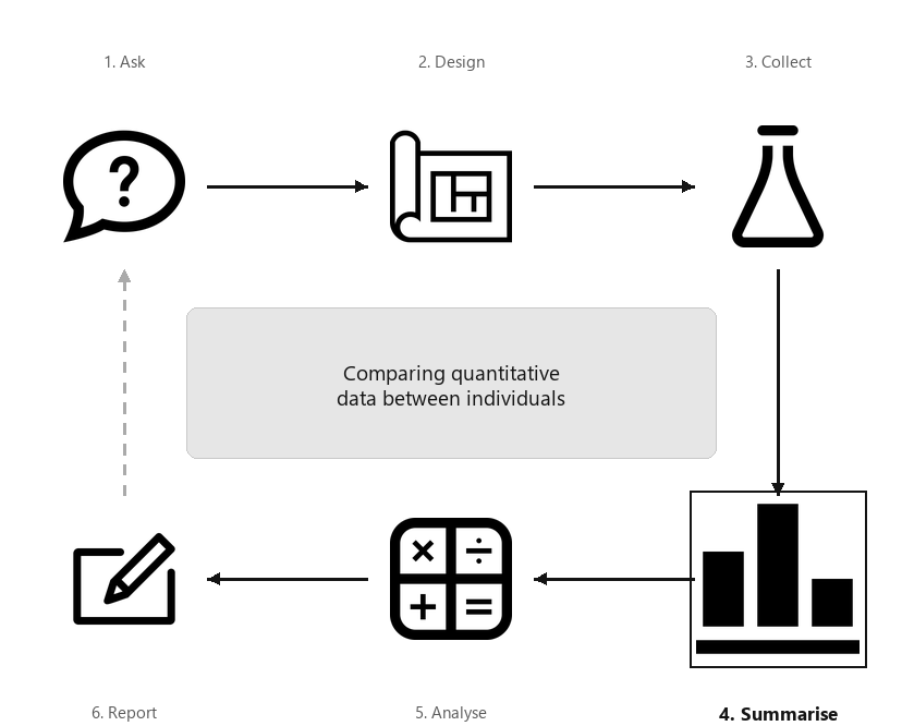
A diagram showing the six steps of research, arranged in a cycle: Ask, Design, Collect, Classify and summarise, Analyse, Report. Step 4 (Summarise) is highlighted, captioned “Comparing quantitative data between individuals”.
Relational RQs compare groups. This chapter considers how to compare quantitative variables in different groups. Graphs are useful this purpose, and a table of the numerical summaries usually is produced also.
When comparing quantitative variables in different groups, the data should be summarised for each group. If two groups are being compared, the difference between the means and/or medians of the two groups must also be computed. If more than two groups are being compared, the differences between one of the group means/medians (the first, or the benchmark, or the initial situation as the reference level) and the other group means/medians are also usually computed.
[107] recorded the number of chest-beats by gorillas (Table Table 14.2), for gorillas under \(20\) years old (’younger’) and \(20\) years and over (’older’). A summary of the data can be tabulated as in Table Table 14.3. Notice that no standard deviation or sample size is provided for the difference; these make no sense.
When a quantitative variable is measured or observed in different groups (i.e., between individuals), the distribution of each variable can be graphed separately. However, to compare the quantitative variable in the groups, appropriate graphs include:
Back-to-back stemplots are two stemplots (Sect. Subsection 11.3.2) sharing the same stems; one group has the leaves emerging left-to-right from the stem, and the second group has the leaves emerging right-to-left from the stem. Back-to-back stemplots can only be used when two groups are being compared. Again, one advantage of using stemplots over other plots is that the original data are retained. Disadvantages are that only two groups can be compared, and not all data work well with stemplots.
A back-to-back stemplot for comparing the chest-beating rate of gorillas (Fig. Figure 14.5) has the leaves for younger gorillas right-to-left, and the leaves for older gorillas left-to-right, sharing the same stems. The younger gorillas have a faster chest-beating rate in general. One older gorilla has a much faster rate than the other older gorillas (a potential outlier).
A two-dimensional (2-D) dot chart places a dot for each observation, separated for each level of the qualitative variable (also see Sect. Subsection 12.3.1). Any number of groups can be compared.
The axis displaying the counts (or percentages) need not start from zero, since the distance from the axis to the these numbers do not visually imply any quantity of interest. Rather, how the dots compare in the groups is the main feature of interest.
For the chest-beating data seen in Example Example 14.4, a dot chart is shown in Fig. Figure 14.8. Many observations are the same, so some points would be overplotted if points were not stacked (left panel), or jittered (right panel).
A boxplot is a picture of the quantiles (Sect. Subsection 11.7.3) for each group, drawn side-by-side on the same plot (and so are sometimes called parallel boxplots or side-by-side boxplots). Any number of groups can be compared using a boxplot. Sometimes, the mean of each groups is added to the boxplot using, for example, a solid dot.
The distribution for each group is summarised by five numbers: the minimum value; the first quartile (\(Q_1\)); the median (\(Q_2\)); the third quartile (\(Q_3\)); and the maximum value. Outliers, identified using the IQR rule (Sect. Subsection 11.8.2), are usually shown too. The values of \(Q_1\text{,}\) the median, and \(Q_3\) for each group can be used to compare the distributions. Different software may use different rules for computing quartiles, and hence may produce slightly different boxplots.
The axis displaying these five numbers need not start from zero, since the distance from the axis to the these numbers do not visually imply any quantity of interest. Rather, the boxes display the values of these five numbers for each group relative to each other, which is of interest.
Boxplots summarise data with only five numbers (sometimes called the five-number summary), so details of the distributions are lost. For this reason, boxplots are excellent for comparing distributions, but histograms are better for displaying the distribution of a single quantitative variable.
The boxplot for the chest-beating data (Example Example 14.4) is shown in Fig. Figure 14.12. No outliers are identified for younger gorillas; one large outlier is identified for the older gorillas. The boxplot shows a distinct difference between the chest-beating rates of older and younger gorillas.
The detail of the boxplots are explained in Fig. Figure 14.13. Firstly, focus on just the boxplot for the younger gorillas (i.e., the left box). Boxplots have five horizontal lines.
Second line from top: \(75\)% of observations are smaller than about \(2.9\) per \(10\) h, represented by the line at the top of the central box. This is the third quartile (\(Q_3\)).
Middle line: \(50\)% of observations are smaller than about \(1.7\) per \(10\) h, represented by the line inside the central box. This is the median value, the second quartile (\(Q_2\)).
Second line from bottom: \(25\)% of observations are smaller than about \(1.5\) per \(10\) h, represented by the line at the bottom of the central box. This is the first quartile (\(Q_1\)).
The box for the older gorillas (Fig. Figure 14.12, right box) is slightly different: one observation is identified with a point, above the top line. Computer software identifies this observation as an extreme outlier using the IQR rule (Sect. Subsection 11.8.2), and has plotted this point separately.
The values of \(Q_1\text{,}\) the median and \(Q_3\) are all substantially larger for the younger gorillas, suggesting that younger gorillas have, in general, faster chest-beating rates.
Boxplots can be plotted horizontally too, which leaves space for long labels of the qualitative variable. In Fig. Figure 14.15 (based on [125]), the three dental cements are very different regarding their push-out forces.
[119] recorded data about access to water in three rural communities in Cameroon (Sect. Section 11.10). The study could be used to determine associations to the incidence of diarrhoea in young children (\(85\) households had children under \(5\) years of age).
The graphs (Fig. Figure 14.16) and summary (Table Table 14.17) show that households in which diarrhoea was found in the last two weeks in children had older household coordinators, more people in the household, and more children under \(5\) years of age in the household. These may be expected: older female coordinators probably have more children, hence more children in the household under \(5\text{,}\) and so more children (and so people) are in the household in general.
Figure14.16.Three plots for the water access data in 85 households (59 household reported no diarrhoea in children under 5 years of age; 26 reported diarrhoea in children under 5 years of age).
Table14.17.A summary of the quantitative variables in the water-access study, according to whether diarrhoea had been observed in the last two weeks in children under \(5\) years of age.
Quantitative data can be compared between different groups (between individuals comparisons) using a back-to-back stemplot, boxplot or \(2\)-D dot chart. A summary table should show the numerical summaries for the levels of the quantitative variable, and the between-group differences.
[123] studied two different engineering project delivery methods (Fig. Figure 14.18, left panel): Design/Build and Design/Bid/Build. The grey, horizontal line is where the projected costs are the same as the actual cost.
[Dataset: AISsub] [126] studied athletes at the Australian Institute of Sport (AIS). Numerous physical and blood measurements were taken from high performance athletes. Figure Figure 14.18 (right panel) compares the heights of females in two similar sports: basketball and netball. (Netball was derived from basketball.)
Figure14.18.Left: cost increases for two different building project delivery methods: Design/Build and Design/Bid/Build (the grey, horizontal line is where the projected costs are the same as the actual cost). Right: the heights of female basketball and netball players attending the AIS.
For which datasets would the mean and standard deviation be the appropriate numerical summary? For which datasets would the median and IQR be the appropriate numerical summary?
[128][113] compared the dimensions of jellyfish at two sites at Hawkesbury River, NSW (Dangar Island; Salamander Bay) to determine the difference between the jellyfish at each site. A histogram of the breadth of jellyfish at Dangar Island Bay is shown in Fig. Figure 14.20 (left panel).
Two students are arguing about the median breadth. Student 1 says: The bars in the histogram have heights of \(10\text{,}\)\(2\text{,}\)\(4\text{,}\)\(2\) and \(4\text{.}\) When these numbers are put in order, they are: \(2\text{,}\)\(2\text{,}\)\(4\text{,}\)\(4\text{,}\) and \(10\text{.}\) The median breadth is the median of these numbers, so the median breadth is the middle one: \(4\) is the median. Student 2 responds: You have the correct answer, but for the wrong reason! There are five bars, and the middle bar is the third bar. Since the third bar has a height of \(4\text{,}\) the median breadth is \(4\text{.}\) Which student, if either, is correct?
A boxplot comparing the breadths of jellyfish at Dangar Island and Salamander Bay is shown in Fig. Figure 14.20 (right panel). Describe and compare the breadths of the jellyfish.
[122] studied the productivity of construction workers, recording (among other variables) the rate at which concrete panels could be installed by workers. Data for three different female workers in the study are shown in Table Table 14.21, gathered over four installation periods of \(50\) min each.
In a study of the temperature in offices, [124] compared the temperature in three offices (during working hours) at Charles Sturt University (Australia; CSU); the data are summarised in Table Table 14.22.
Table14.22.A summary of the temperature (in degrees C) in three offices at CSU during working hours. Office A is on the ground floor; Offices B and C are on the top floor.
[Dataset: ForwardFall] [127] compared the lean-forward angle in younger and older women. An elaborate set-up was constructed to measure this angle, using a harness. Consider the RQ:
[Dataset: Speed] [120] studied adding additional signage to reduce vehicle speeds on freeway exit ramps. At one site (Ningxuan Freeway), speeds were recorded for \(38\) vehicles before the extra signage was added, and then for \(41\) different vehicles after the extra signage was added.
[Dataset: Deceleration] [120] studied adding additional signage to reduce vehicle speeds on freeway exit ramps. At one site (Ningxuan Freeway), speeds were recorded at various points on the freeway exit for \(38\) vehicles before the extra signage was added, and then for \(41\) vehicles after the extra signage was added.
From this data, the deceleration of each vehicle was determined as the vehicle left the \(120\) km.h\(^{-1}\) speed zone and approached the \(80\) km.h\(^{-1}\) speed zone. The RQ is:
At this freeway exit, what is the difference between the mean vehicle deceleration, comparing the times before the extra signage is added and after extra signage is added?
In this context, the researchers are hoping that the extra signage might cause cars to slow down faster (i.e., they will decelerate more, on average, after adding the extra signage).
[Dataset: Typing] The Typing dataset contains information about the typing speed and accuracy for students, from an online typing test [69]. The four variables are: typing speed (mTS), typing accuracy (mAcc), age (Age), and sex (Sex) for \(1 301\) students.
[Dataset: Dental] [129] recorded the sugar consumption and the average number of decayed, missing or filled teeth (DMFT) in \(29\) industrialised countries and \(61\) non-industrialised countries.
[Dataset: Snakes] Some Mexican garter snakes (Thamnophis melanogaster) live in habitats with no crayfish, while some live in habitats with crayfish and use crayfish as a food source. [121] were interested in whether the snakes in these regions were different: