Power calculations for a difference of means

Section 7.4 Power calculations for a difference of means

Often times in experiment planning, there are two competing considerations:

We want to collect enough data that we can detect important effects.
🔗

🔗
Collecting data can be expensive, and in experiments involving people, there may be some risk to patients.
🔗

🔗

In this section, we focus on the context of a clinical trial, which is a health-related experiment where the subject are people, and we will determine an appropriate sample size where we can be 80% sure that we would detect any practically important effects.

Even though we don’t cover it explicitly, similar sample size planning is also helpful for observational studies.

🔗

Subsection 7.4.1 Going through the motions of a test

We’re going to go through the motions of a hypothesis test. This will help us frame our calculations for determining an appropriate sample size for the study.

🔗

Example 7.4.1.

Suppose a pharmaceutical company has developed a new drug for lowering blood pressure, and they are preparing a clinical trial (experiment) to test the drug’s effectiveness. They recruit people who are taking a particular standard blood pressure medication. People in the control group will continue to take their current medication through generic-looking pills to ensure blinding. Write down the hypotheses for a two-sided hypothesis test in this context.

🔗

Solution.

Generally, clinical trials use a two-sided alternative hypothesis, so below are suitable hypotheses for this context:

\(H_0\text{:}\) 🔗: The new drug performs exactly as well as the standard medication. \(\mu_{trmt} - \mu_{ctrl} = 0\text{.}\)
🔗
\(H_A\text{:}\) 🔗: The new drug’s performance differs from the standard medication. \(\mu_{trmt} - \mu_{ctrl} \neq 0\text{.}\)
🔗

🔗

Example 7.4.2.

The researchers would like to run the clinical trial on patients with systolic blood pressures between 140 and 180 mmHg. Suppose previously published studies suggest that the standard deviation of the patients’ blood pressures will be about 12 mmHg and the distribution of patient blood pressures will be approximately symmetric.

In this particular study, we’d generally measure each patient’s blood pressure at the beginning and end of the study, and then the outcome measurement for the study would be the average change in blood pressure. That is, both \(\mu_{trmt}\) and \(\mu_{ctrl}\) would represent average differences. This is what you might think of as a 2-sample paired testing structure, and we’d analyze it exactly just like a hypothesis test for a difference in the average change for patients. In the calculations we perform here, we’ll suppose that 12 mmHg is the predicted standard deviation of a patient’s blood pressure difference over the course of the study.

If we had 100 patients per group, what would be the approximate standard error for \(\bar{x}_{trmt} - \bar{x}_{ctrl}\text{?}\)

🔗

Solution.

The standard error is calculated as follows:

\begin{align*} SE_{\bar{x}_{trmt} - \bar{x}_{ctrl}} \amp = \sqrt{\frac{s_{trmt}^2}{n_{trmt}} + \frac{s_{ctrl}^2}{n_{ctrl}}}\\ \amp = \sqrt{\frac{12^2}{100} + \frac{12^2}{100}}\\ \amp = 1.70 \end{align*}

This may be an imperfect estimate of \(SE_{\bar{x}_{trmt} - \bar{x}_{ctrl}}\text{,}\) since the standard deviation estimate we used may not be perfectly correct for this group of patients. However, it is sufficient for our purposes.

🔗

Example 7.4.3.

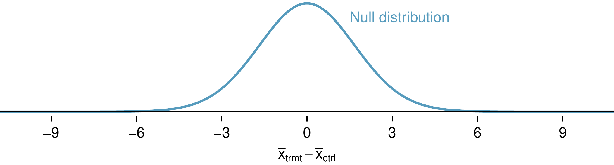
What does the null distribution of \(\bar{x}_{trmt} - \bar{x}_{ctrl}\) look like?

🔗

Solution.

The degrees of freedom are greater than 30, so the distribution of \(\bar{x}_{trmt} - \bar{x}_{ctrl}\) will be approximately normal. The standard deviation of this distribution (the standard error) would be about 1.70, and under the null hypothesis, its mean would be 0.

🔗

A normal distribution is shown for "x-bar-sub-treatment minus x-bar-sub-control", where the distribution is centered at zero and has a standard deviation of about 1.6. The distribution is labeled as "Null distribution". — Figure 7.4.4.
🔗

🔗

Example 7.4.5.

For what values of \(\bar{x}_{trmt} - \bar{x}_{ctrl}\) would we reject the null hypothesis?

🔗

Solution.

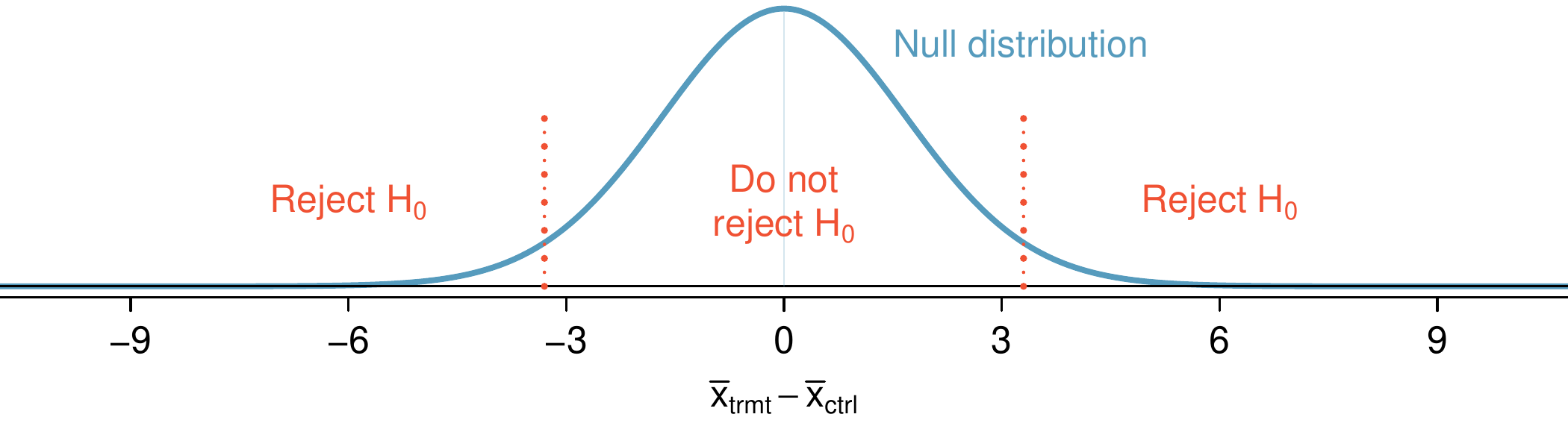
For \(\alpha = 0.05\text{,}\) we would reject \(H_0\) if the difference is in the lower 2.5% or upper 2.5% tail:

Lower 2.5%: 🔗: For the normal model, this is 1.96 standard errors below 0, so any difference smaller than \(-1.96 \times 1.70 = -3.332\) mmHg.
🔗
Upper 2.5%: 🔗: For the normal model, this is 1.96 standard errors above 0, so any difference larger than \(1.96 \times 1.70 = 3.332\) mmHg.
🔗

The boundaries of these rejection regions are shown below:

🔗

Next, we’ll perform some hypothetical calculations to determine the probability we reject the null hypothesis, if the alternative hypothesis were actually true.

🔗

Subsection 7.4.2 Computing the power for a 2-sample test

When planning a study, we want to know how likely we are to detect an effect we care about. In other words, if there is a real effect, and that effect is large enough that it has practical value, then what’s the probability that we detect that effect? This probability is called the power, and we can compute it for different sample sizes or for different effect sizes.

🔗

We first determine what is a practically significant result. Suppose that the company researchers care about finding any effect on blood pressure that is 3 mmHg or larger vs the standard medication. Here, 3 mmHg is the minimum effect size of interest, and we want to know how likely we are to detect this size of an effect in the study.

🔗

Example 7.4.7.

Suppose we decided to move forward with 100 patients per treatment group and the new drug reduces blood pressure by an additional 3 mmHg relative to the standard medication. What is the probability that we detect a drop?

🔗

Solution.

Before we even do any calculations, notice that if \(\bar{x}_{trmt} - \bar{x}_{ctrl} = -3\) mmHg, there wouldn’t even be sufficient evidence to reject \(H_0\text{.}\) That’s not a good sign.

🔗

To calculate the probability that we will reject \(H_0\text{,}\) we need to determine a few things:

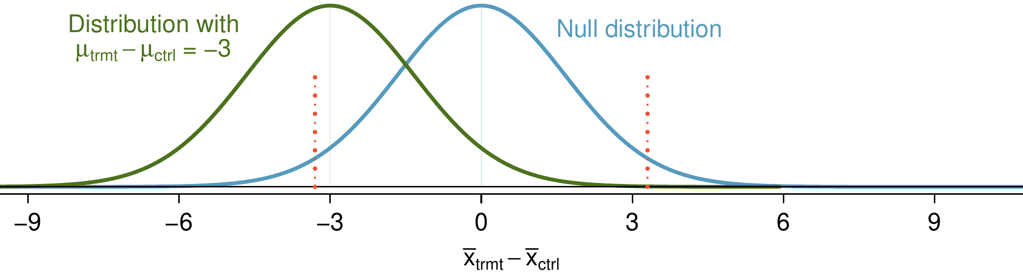
The sampling distribution for \(\bar{x}_{trmt} - \bar{x}_{ctrl}\) when the true difference is -3 mmHg. This is the same as the null distribution, except it is shifted to the left by 3:
🔗

Figure 7.4.8.
🔗

🔗
The rejection regions, which are outside of the dotted lines above.
🔗

🔗
The fraction of the distribution that falls in the rejection region.
🔗

🔗

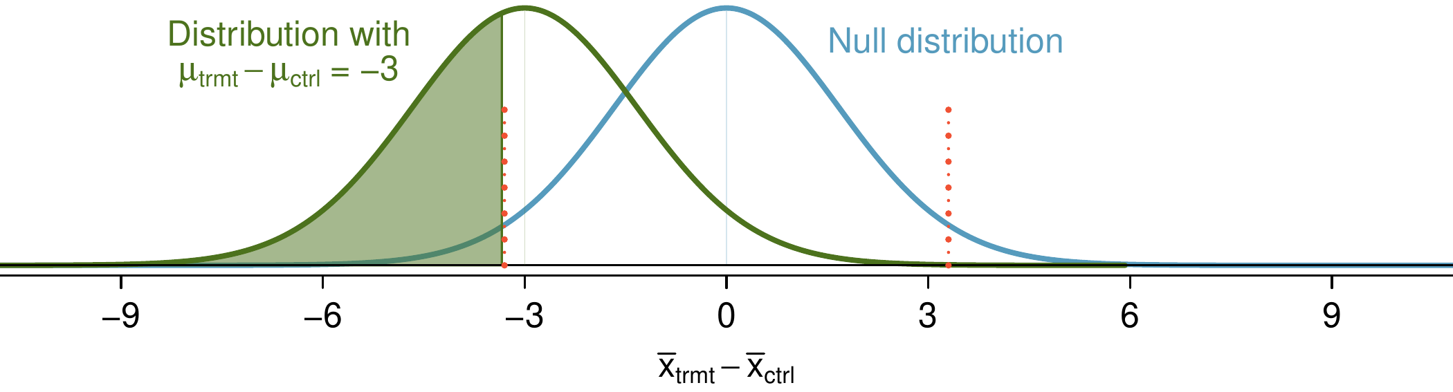
In short, we need to calculate the probability that \(x \lt -3.332\) for a normal distribution with mean -3 and standard deviation 1.7. To do so, we first shade the area we want to calculate:

🔗

We’ll use a normal approximation, which is good approximation when the degrees of freedom is about 30 or more. We’ll start by calculating the Z-score and find the tail area using either statistical software or the probability table:

\begin{gather*} Z = \frac{-3.332 - (-3)}{1.7} = -0.20 \qquad \to \qquad 0.42 \end{gather*}

The power for the test is about 42% when \(\mu_{trmt} - \mu_{ctrl} = -3\) and each group has a sample size of 100.

🔗

In Example 7.4.7, we ignored the upper rejection region in the calculation, which was in the opposite direction of the hypothetical truth, i.e. -3. The reasoning? There wouldn’t be any value in rejecting the null hypothesis and concluding there was an increase when in fact there was a decrease.

🔗

We’ve also used a normal distribution instead of the \(t\)-distribution. This is a convenience, and if the sample size is too small, we’d need to revert back to using the \(t\)-distribution. We’ll discuss this a bit further at the end of this section.

🔗

Subsection 7.4.3 Determining a proper sample size

In the last example, we found that if we have a sample size of 100 in each group, we can only detect an effect size of 3 mmHg with a probability of about 0.42. Suppose the researchers moved forward and only used 100 patients per group, and the data did not support the alternative hypothesis, i.e. the researchers did not reject \(H_0\text{.}\) This is a very bad situation to be in for a few reasons:

In the back of the researchers’ minds, they’d all be wondering, maybe there is a real and meaningful difference, but we weren’t able to detect it with such a small sample.
🔗

🔗
The company probably invested hundreds of millions of dollars in developing the new drug, so now they are left with great uncertainty about its potential since the experiment didn’t have a great shot at detecting effects that could still be important.
🔗

🔗
Patients were subjected to the drug, and we can’t even say with much certainty that the drug doesn’t help (or harm) patients.
🔗

🔗
Another clinical trial may need to be run to get a more conclusive answer as to whether the drug does hold any practical value, and conducting a second clinical trial may take years and many millions of dollars.
🔗

🔗

We want to avoid this situation, so we need to determine an appropriate sample size to ensure we can be pretty confident that we’ll detect any effects that are practically important. As mentioned earlier, a change of 3 mmHg was deemed to be the minimum difference that was practically important. As a first step, we could calculate power for several different sample sizes. For instance, let’s try 500 patients per group.

🔗

Checkpoint 7.4.10.

Calculate the power to detect a change of -3 mmHg when using a sample size of 500 per group.

Determine the standard error (recall that the standard deviation for patients was expected to be about 12 mmHg).
🔗

🔗
Identify the null distribution and rejection regions.
🔗

🔗
Identify the alternative distribution when \(\mu_{trmt} - \mu_{ctrl} = -3\text{.}\)
🔗

🔗
Compute the probability we reject the null hypothesis.
🔗

🔗

🔗

Solution.

(a) The standard error is given as \(SE = \sqrt{\frac{12^2}{500} + \frac{12^2}{500}} = 0.76\text{.}\)

🔗

(b) & (c) The null distribution, rejection boundaries, and alternative distribution are shown below:

🔗

The rejection regions are the areas on the outside of the two dotted lines and are at \(\pm 0.76 \times 1.96 = \pm 1.49\text{.}\)

🔗

(d) The area of the alternative distribution where \(\mu_{trmt} - \mu_{ctrl} = -3\) has been shaded. We compute the Z-score and find the tail area: \(Z = \frac{-1.49 - (-3)}{0.76} = 1.99 \to 0.977\text{.}\) With 500 patients per group, we would be about 97.7% sure (or more) that we’d detect any effects that are at least 3 mmHg in size.

🔗

The researchers decided 3 mmHg was the minimum difference that was practically important, and with a sample size of 500, we can be very certain (97.7% or better) that we will detect any such difference. We now have moved to another extreme where we are exposing an unnecessary number of patients to the new drug in the clinical trial. Not only is this ethically questionable, but it would also cost a lot more money than is necessary to be quite sure we’d detect any important effects.

🔗

The most common practice is to identify the sample size where the power is around 80%, and sometimes 90%. Other values may be reasonable for a specific context, but 80% and 90% are most commonly targeted as a good balance between high power and not exposing too many patients to a new treatment (or wasting too much money).

🔗

We could compute the power of the test at several other possible sample sizes until we find one that’s close to 80%, but there’s a better way. We should solve the problem backwards.

🔗

Example 7.4.12.

What sample size will lead to a power of 80%? Use \(\alpha = 0.05\text{.}\)

🔗

Solution.

We’ll assume we have a large enough sample that the normal distribution is a good approximation for the test statistic, since the normal distribution and the \(t\)-distribution look almost identical when the degrees of freedom are moderately large (e.g. \(df \geq 30\)). If that doesn’t turn out to be true, then we’d need to make a correction.

🔗

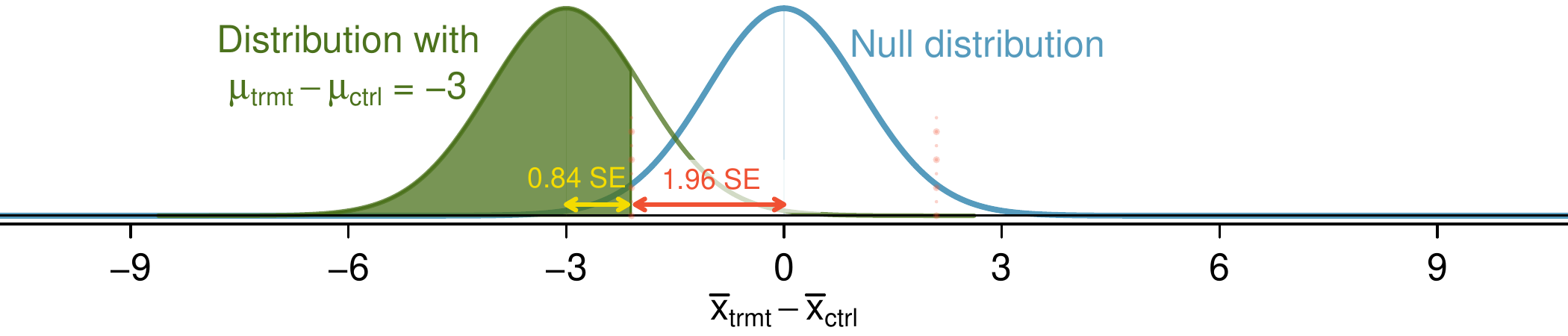
We start by identifying the Z-score that would give us a lower tail of 80%. For a moderately large sample size per group, the Z-score for a lower tail of 80% would be about \(Z = 0.84\text{.}\)

🔗

Additionally, the rejection region extends \(1.96\times SE\) from the center of the null distribution for \(\alpha = 0.05\text{.}\) This allows us to calculate the target distance between the center of the null and alternative distributions in terms of the standard error:

\begin{gather*} 0.84 \times SE + 1.96 \times SE = 2.8 \times SE \end{gather*}

In our example, we want the distance between the null and alternative distributions’ centers to equal the minimum effect size of interest, 3 mmHg, which allows us to set up an equation between this difference and the standard error:

\begin{align*} 3 \amp = 2.8 \times SE\\ 3 \amp = 2.8 \times \sqrt{\frac{12^2}{n} + \frac{12^2}{n}}\\ n \amp = \frac{2.8^2}{3^2} \times \left( 12^2 + 12^2 \right) = 250.88 \end{align*}

We should target 251 patients per group in order to achieve 80% power at the 0.05 significance level for this context.

🔗

The standard error difference of \(2.8 \times SE\) is specific to a context where the targeted power is 80% and the significance level is \(\alpha = 0.05\text{.}\) If the targeted power is 90% or if we use a different significance level, then we’ll use something a little different than \(2.8 \times SE\text{.}\)

🔗

Had the suggested sample size been relatively small -- roughly 30 or smaller -- it would have been a good idea to rework the calculations using the degrees of fredom for the smaller sample size under that initial sample size. That is, we would have revised the 0.84 and 1.96 values based on degrees of freedom implied by the initial sample size. The revised sample size target would generally have then been a little larger.

🔗

Checkpoint 7.4.14.

Suppose the targeted power was 90% and we were using \(\alpha = 0.01\text{.}\) How many standard errors should separate the centers of the null and alternative distribution, where the alternative distribution is centered at the minimum effect size of interest?

🔗

Solution.

First, find the Z-score such that 90% of the distribution is below it: \(Z = 1.28\text{.}\) Next, find the cutoffs for the rejection regions: \(\pm 2.58\text{.}\) Then the difference in centers should be about \(1.28 \times SE + 2.58 \times SE = 3.86 \times SE\text{.}\)

🔗

Checkpoint 7.4.15.

What are some considerations that are important in determining what the power should be for an experiment?

🔗

Solution.

Answers will vary, but here are a few important considerations:

Whether there is any risk to patients in the study.
🔗

🔗
The cost of enrolling more patients.
🔗

🔗
The potential downside of not detecting an effect of interest.
🔗

🔗

🔗

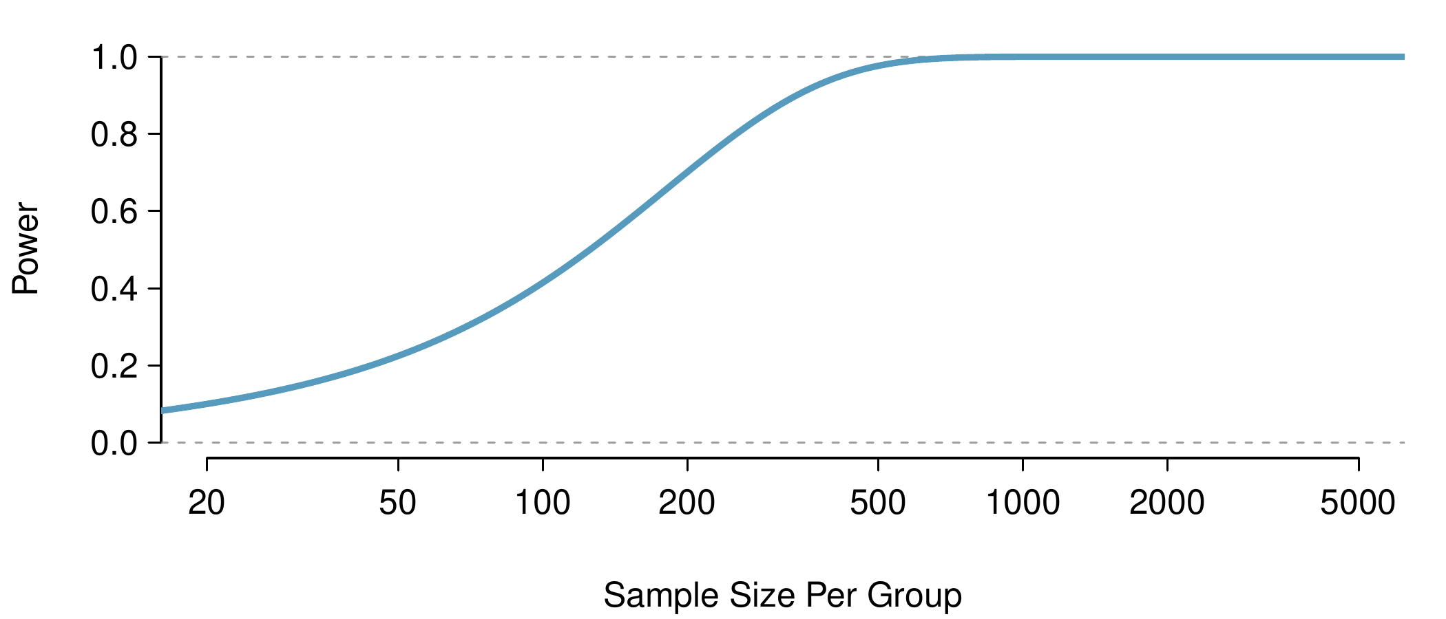
Figure 7.4.16 shows the power for sample sizes from 20 patients to 5,000 patients when \(\alpha = 0.05\) and the true difference is -3. This curve was constructed by writing a program to compute the power for many different sample sizes.

🔗

A line plot is shown with "Sample Size Per Group" on the horizontal axis and "Power" on the vertical axis. The horizontal axis values grow exponentially and has values going from 20 to 50 to 100 to 200 to 500 to 1,000 to 2,000 and finally to 5,000. The line starts at about (20, 0.1) and slowly climbs up to about (50, 0.25), then climbs more quickly up to (100, 0.4), then (200, 0.7), where its growth starts tapering off as nearly flattens at about (500, 0.98). The height of the line is indistinguishable from 1 for sample sizes per group of 1,000 and higher. — Figure 7.4.16. The curve shows the power for different sample sizes in the context of the blood pressure example when the true difference is -3. Having more than about 250 to 350 observations doesn’t provide much additional value in detecting an effect when \(\alpha = 0.05\text{.}\)
🔗

Power calculations for expensive or risky experiments are critical. However, what about experiments that are inexpensive and where the ethical considerations are minimal? For example, if we are doing final testing on a new feature on a popular website, how would our sample size considerations change? As before, we’d want to make sure the sample is big enough. However, suppose the feature has undergone some testing and is known to perform well (e.g. the website’s users seem to enjoy the feature). Then it may be reasonable to run a larger experiment if there’s value from having a more precise estimate of the feature’s effect, such as helping guide the development of the next useful feature.

🔗

Exercises 7.4.4 Exercises

1. Increasing corn yield..

Increasing corn yield. A large farm wants to try out a new type of fertilizer to evaluate whether it will improve the farm’s corn production. The land is broken into plots that produce an average of 1,215 pounds of corn with a standard deviation of 94 pounds per plot. The owner is interested in detecting any average difference of at least 40 pounds per plot. How many plots of land would be needed for the experiment if the desired power level is 90%? Use \(\alpha = 0.05\text{.}\) Assume each plot of land gets treated with either the current fertilizer or the new fertilizer.

🔗

2. Email outreach efforts..

Email outreach efforts. A medical research group is recruiting people to complete short surveys about their medical history. For example, one survey asks for information on a person’s family history in regards to cancer. Another survey asks about what topics were discussed during the person’s last visit to a hospital. So far, as people sign up, they complete an average of just 4 surveys, and the standard deviation of the number of surveys is about 2.2. The research group wants to try a new interface that they think will encourage new enrollees to complete more surveys, where they will randomize each enrollee to either get the new interface or the current interface. How many new enrollees do they need for each interface to detect an effect size of 0.5 surveys per enrollee, if the desired power level is 80%? Use \(\alpha = 0.05\text{.}\)

🔗

Prev Top Next