Case study: malaria vaccine

Section 2.3 Case study: malaria vaccine

Example 2.3.1. Class seating and Apple ownership.

Suppose your professor splits the students in class into two groups: students on the left and students on the right. If \(\hat{p}_L\) and \(\hat{p}_R\) represent the proportion of students who own an Apple product on the left and right, respectively, would you be surprised if \(\hat{p}_L\) did not exactly equal \(\hat{p}_R\text{?}\)

🔗

Solution.

While the proportions would probably be close to each other, it would be unusual for them to be exactly the same. We would probably observe a small difference due to chance.

🔗

Checkpoint 2.3.2. Independence between seating and ownership.

If we don’t think the side of the room a person sits on in class is related to whether the person owns an Apple product, what assumption are we making about the relationship between these two variables?

🔗

Solution.

We would be assuming that these two variables are independent.

🔗

Subsection 2.3.1 Variability within data

We consider a study on a new malaria vaccine called PfSPZ. In this study, volunteer patients were randomized into one of two experiment groups: 14 patients received an experimental vaccine and 6 patients received a placebo vaccine. Nineteen weeks later, all 20 patients were exposed to a drug-sensitive malaria parasite strain; the motivation of using a drug-sensitive strain of parasite here is for ethical considerations, allowing any infections to be treated effectively. The results are summarized in Table 2.3.3, where 9 of the 14 treatment patients remained free of signs of infection while all of the 6 patients in the control group patients showed some baseline signs of infection.

🔗

Table 2.3.3. Summary results for the malaria vaccine experiment

🔗

		`outcome`		Total
		infection	no infection
`treatment`	vaccine	5	9	14
placebo	6	0	6
	Total	11	9	20

Checkpoint 2.3.4. Study design and implications.

Is this an observational study or an experiment? What implications does the study type have on what can be inferred from the results?

🔗

Solution.

The study is an experiment, as patients were randomly assigned an experiment group. Since this is an experiment, the results can be used to evaluate a causal relationship between the malaria vaccine and whether patients showed signs of an infection.

🔗

In this study, a smaller proportion of patients who received the vaccine showed signs of an infection (35.7% versus 100%). However, the sample is very small, and it is unclear whether the difference provides convincing evidence that the vaccine is effective.

🔗

Example 2.3.5. Assessing the evidence.

Data scientists are sometimes called upon to evaluate the strength of evidence. When looking at the rates of infection for patients in the two groups in this study, what comes to mind as we try to determine whether the data show convincing evidence of a real difference?

🔗

Solution.

The observed infection rates (35.7% for the treatment group versus 100% for the control group) suggest the vaccine may be effective. However, we cannot be sure if the observed difference represents the vaccine’s efficacy or is just from random chance. Generally there is a little bit of fluctuation in sample data, and we wouldn’t expect the sample proportions to be exactly equal, even if the truth was that the infection rates were independent of getting the vaccine. Additionally, with such small samples, perhaps it’s common to observe such large differences when we randomly split a group due to chance alone!

🔗

Example 2.3.5 is a reminder that the observed outcomes in the data sample may not perfectly reflect the true relationships between variables since there is random noise. While the observed difference in rates of infection is large, the sample size for the study is small, making it unclear if this observed difference represents efficacy of the vaccine or whether it is simply due to chance. We label these two competing claims, \(H_0\) and \(H_A\text{,}\) which are spoken as "H-nought" and "H-A":

🔗

\(H_0\text{:}\) Independence model. The variables treatment and outcome are independent. They have no relationship, and the observed difference between the proportion of patients who developed an infection in the two groups, 64.3%, was due to chance.
🔗

🔗
\(H_A\text{:}\) Alternative model. The variables are not independent. The difference in infection rates of 64.3% was not due to chance, and vaccine affected the rate of infection.
🔗

🔗

🔗

What would it mean if the independence model, which says the vaccine had no influence on the rate of infection, is true? It would mean 11 patients were going to develop an infection no matter which group they were randomized into, and 9 patients would not develop an infection no matter which group they were randomized into. That is, if the vaccine did not affect the rate of infection, the difference in the infection rates was due to chance alone in how the patients were randomized.

🔗

Now consider the alternative model: infection rates were influenced by whether a patient received the vaccine or not. If this was true, and especially if this influence was substantial, we would expect to see some difference in the infection rates of patients in the groups.

🔗

We choose between these two competing claims by assessing if the data conflict so much with \(H_0\) that the independence model cannot be deemed reasonable. If this is the case, and the data support \(H_A\text{,}\) then we will reject the notion of independence and conclude the vaccine was effective.

🔗

Subsection 2.3.2 Simulating the study

We’re going to implement simulations, where we will pretend we know that the malaria vaccine being tested does not work. Ultimately, we want to understand if the large difference we observed is common in these simulations. If it is common, then maybe the difference we observed was purely due to chance. If it is very uncommon, then the possibility that the vaccine was helpful seems more plausible.

🔗

Table 2.3.3 shows that 11 patients developed infections and 9 did not. For our simulation, we will suppose the infections were independent of the vaccine and we were able to rewind back to when the researchers randomized the patients in the study. If we happened to randomize the patients differently, we may get a different result in this hypothetical world where the vaccine doesn’t influence the infection. Let’s complete another randomization using a simulation.

🔗

In this simulation, we take 20 notecards to represent the 20 patients, where we write down "infection" on 11 cards and "no infection" on 9 cards. In this hypothetical world, we believe each patient that got an infection was going to get it regardless of which group they were in, so let’s see what happens if we randomly assign the patients to the treatment and control groups again. We thoroughly shuffle the notecards and deal 14 into a vaccine pile and 6 into a placebo pile. Finally, we tabulate the results, which are shown in Table 2.3.6.

🔗

Table 2.3.6. Simulation results, where any difference in infection rates is purely due to chance

🔗

		`outcome`		Total
		infection	no infection
treatment (simulated)	vaccine	7	7	14
placebo	4	2	6
	Total	11	9	20

Checkpoint 2.3.7. Simulated difference.

What is the difference in infection rates between the two simulated groups in Table 2.3.6? How does this compare to the observed 64.3% difference in the actual data?

🔗

Solution.

\(4/6 - 7/14 = 0.167\) or about 16.7% in favor of the vaccine. This difference due to chance is much smaller than the difference observed in the actual groups.

🔗

Subsection 2.3.3 Checking for independence

We computed one possible difference under the independence model in Guided Practice Checkpoint 2.3.7, which represents one difference due to chance. While in this first simulation, we physically dealt out notecards to represent the patients, it is more efficient to perform this simulation using a computer. Repeating the simulation on a computer, we get another difference due to chance:

\begin{equation*} 2/6 - 9/14 = -0.310 \end{equation*}

And another:

\begin{equation*} 3/6 - 8/14 = -0.071 \end{equation*}

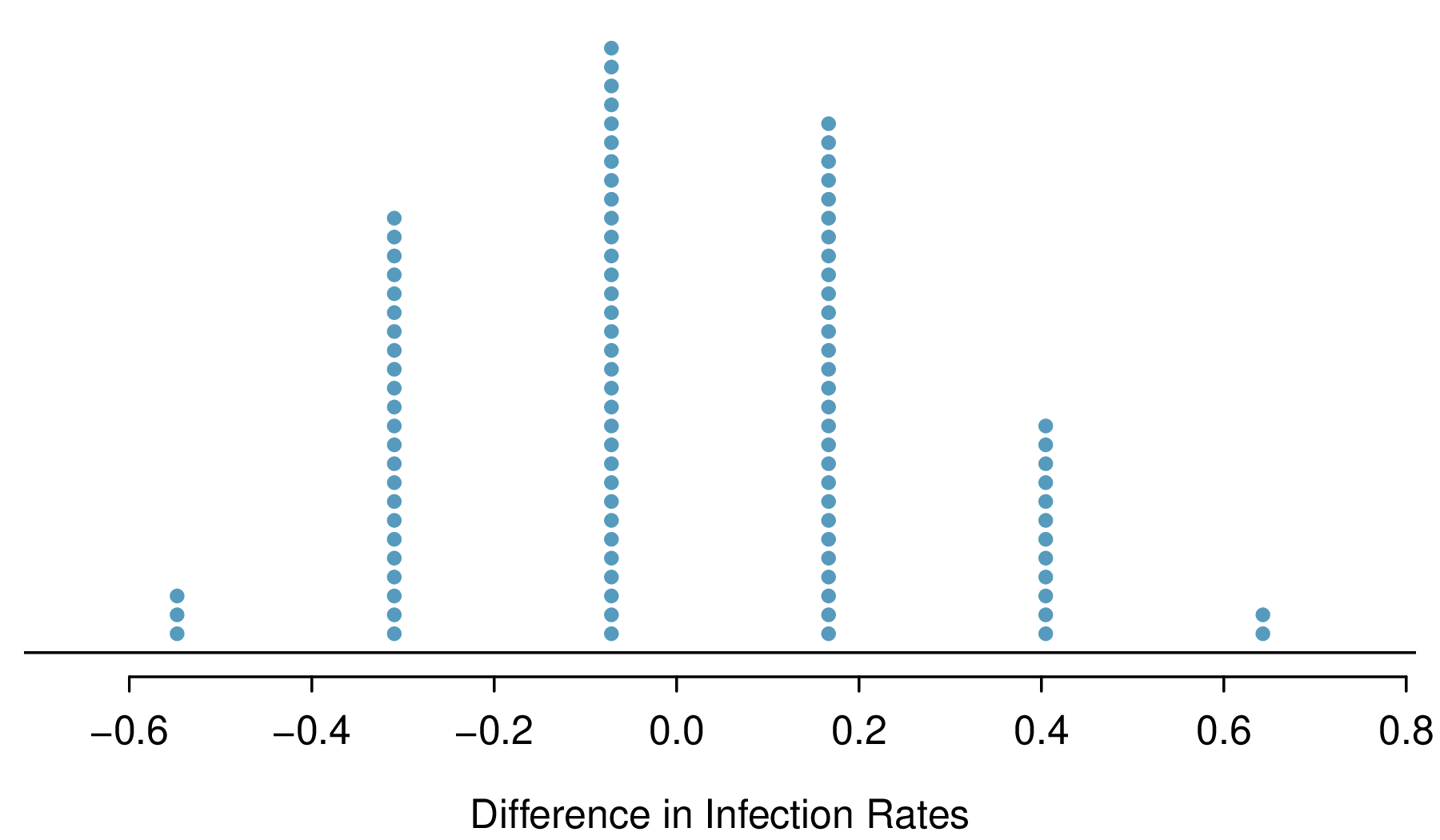
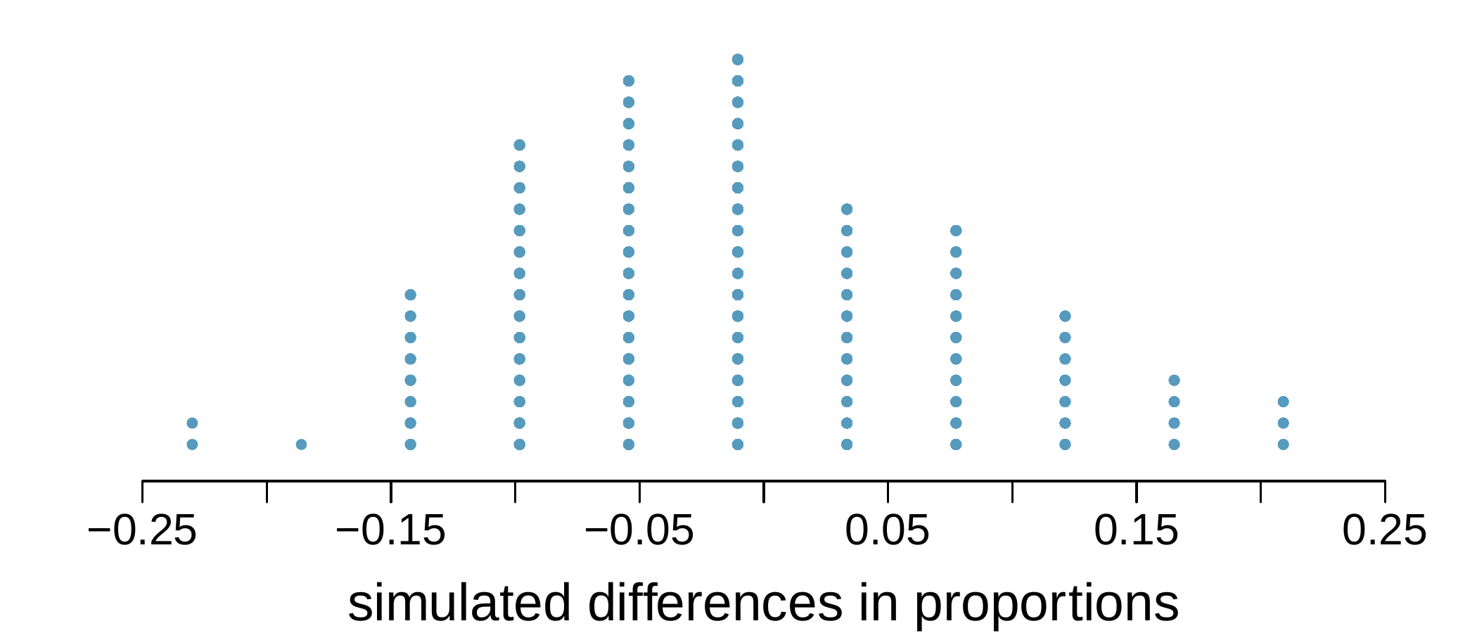
And so on until we repeat the simulation enough times that we have a good idea of what represents the distribution of differences from chance alone. Figure 2.3.8 shows a stacked plot of the differences found from 100 simulations, where each dot represents a simulated difference between the infection rates (control rate minus treatment rate).

🔗

A stacked dot plot is shown. The horizontal axis represents "difference in infection rates" and has a range of -0.6 to 0.8. There are six stacks of dots shown in the plot, with 3 points shown at -0.55, 20-25 points shown at -0.32, 30-35 points shown at -0.08, 25-30 points shown at 0.18, 10-12 points shown at 0.41, and 2 points shown at 0.64. — Figure 2.3.8. Differences from 100 simulations under the independence model
🔗

Note that the distribution of these simulated differences is centered around 0. We simulated these differences assuming that the independence model was true, and under this condition, we expect the difference to be near zero with some random fluctuation, where near is pretty generous in this case since the sample sizes are so small in this study.

🔗

Example 2.3.9. Rarity of the observed difference.

How often would you observe a difference of at least 64.3% (0.643) according to Figure 2.3.8? Often, sometimes, rarely, or never?

🔗

Solution.

It appears that a difference of at least 64.3% due to chance alone would only happen about 2% of the time according to Figure 2.3.8. Such a low probability indicates a rare event.

🔗

The difference of 64.3% being a rare event suggests two possible interpretations of the results of the study:

🔗

\(H_0\text{:}\) Independence model. The vaccine has no effect on infection rate, and we just happened to observe a difference that would only occur on a rare occasion.
🔗

🔗
\(H_A\text{:}\) Alternative model. The vaccine has an effect on infection rate, and the difference we observed was actually due to the vaccine being effective at combatting malaria, which explains the large difference of 64.3%.
🔗

🔗

🔗

Based on the simulations, we have two options. (1) We conclude that the study results do not provide strong evidence against the independence model. That is, we do not have sufficiently strong evidence to conclude the vaccine had an effect in this clinical setting. (2) We conclude the evidence is sufficiently strong to reject \(H_0\) and assert that the vaccine was useful. When we conduct formal studies, usually we reject the notion that we just happened to observe a rare event. So in this case, we reject the independence model in favor of the alternative. That is, we are concluding the data provide strong evidence that the vaccine provides some protection against malaria in this clinical setting.

🔗

One field of statistics, statistical inference, is built on evaluating whether such differences are due to chance. In statistical inference, data scientists evaluate which model is most reasonable given the data. Errors do occur, just like rare events, and we might choose the wrong model. While we do not always choose correctly, statistical inference gives us tools to control and evaluate how often these errors occur. In Chapter 3, we give a formal introduction to the problem of model selection. We spend the next two chapters building a foundation of probability and theory necessary to make that discussion rigorous.

🔗

Exercises 2.3.4 Exercises

1. Side effects of Avandia.

Rosiglitazone is the active ingredient in the controversial type 2 diabetes medicine Avandia and has been linked to an increased risk of serious cardiovascular problems such as stroke, heart failure, and death. A common alternative treatment is pioglitazone, the active ingredient in a diabetes medicine called Actos. In a nationwide retrospective observational study of 227,571 Medicare beneficiaries aged 65 years or older, it was found that 2,593 of the 67,593 patients using rosiglitazone and 5,386 of the 159,978 using pioglitazone had serious cardiovascular problems. These data are summarized in the contingency table below.

🔗

Table 2.3.10. Cardiovascular problems by treatment type

🔗

		Yes	No	Total
Treatment	Rosiglitazone	2,593	65,000	67,593
	Pioglitazone	5,386	154,592	159,978
	Total	7,979	219,592	227,571

Determine if each of the following statements is true or false. If false, explain why. Be careful: The reasoning may be wrong even if the statement’s conclusion is correct. In such cases, the statement should be considered false.
🔗
1. Since more patients on pioglitazone had cardiovascular problems (5,386 vs. 2,593), we can conclude that the rate of cardiovascular problems for those on a pioglitazone treatment is higher.
  🔗
  
  🔗
2. The data suggest that diabetic patients who are taking rosiglitazone are more likely to have cardiovascular problems since the rate of incidence was (2,593 / 67,593 = 0.038) 3.8% for patients on this treatment, while it was only (5,386 / 159,978 = 0.034) 3.4% for patients on pioglitazone.
  🔗
  
  🔗
3. The fact that the rate of incidence is higher for the rosiglitazone group proves that rosiglitazone causes serious cardiovascular problems.
  🔗
  
  🔗
4. Based on the information provided so far, we cannot tell if the difference between the rates of incidences is due to a relationship between the two variables or due to chance.
  🔗
  
  🔗
🔗
What proportion of all patients had cardiovascular problems?
🔗

🔗
If the type of treatment and having cardiovascular problems were independent, about how many patients in the rosiglitazone group would we expect to have had cardiovascular problems?
🔗

🔗
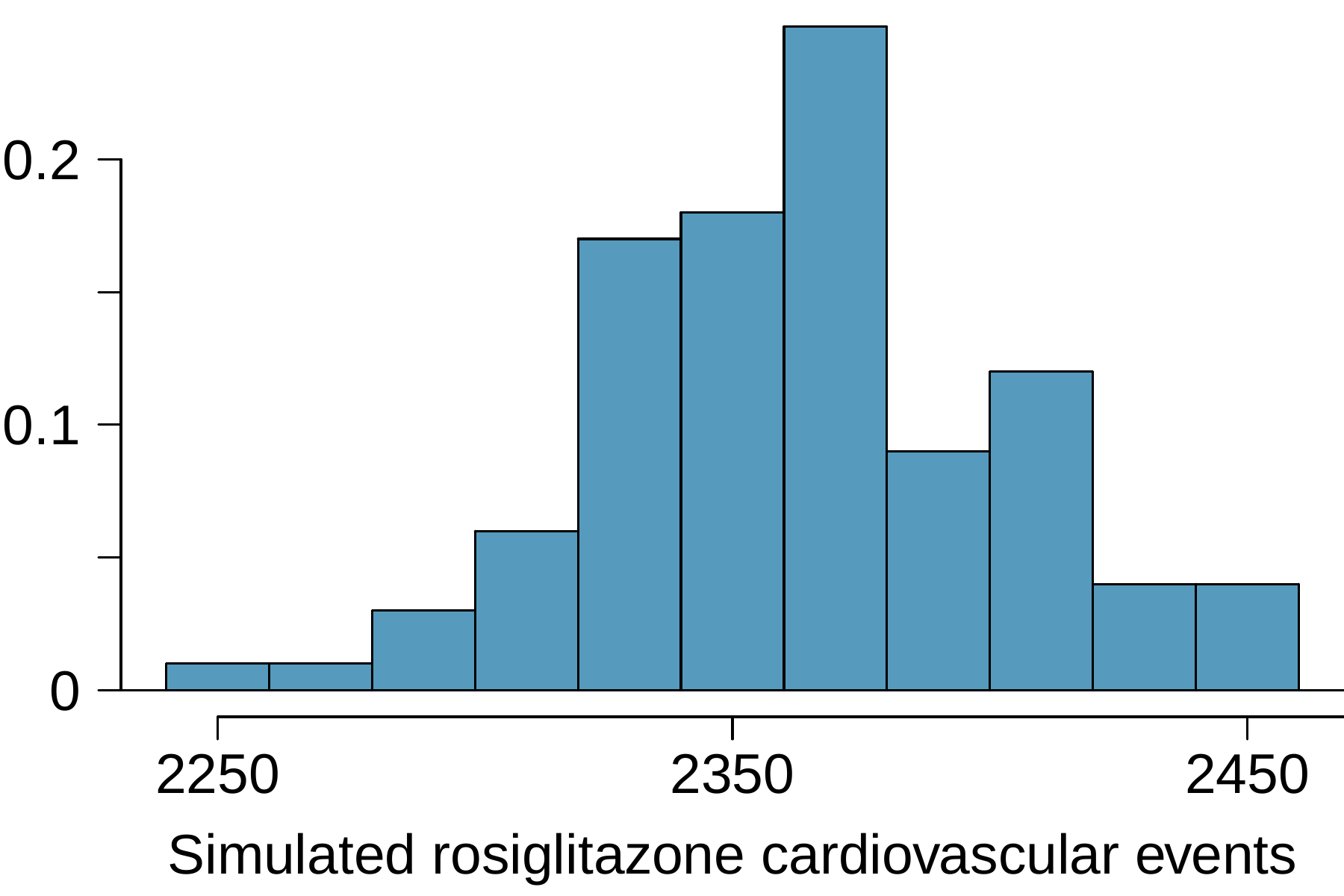
We can investigate the relationship between outcome and treatment in this study using a randomization technique. While in reality we would carry out the simulations required for randomization using statistical software, suppose we actually simulate using index cards. In order to simulate from the independence model, which states that the outcomes were independent of the treatment, we write whether or not each patient had a cardiovascular problem on cards, shuffled all the cards together, then deal them into two groups of size 67,593 and 159,978. We repeat this simulation 1,000 times and each time record the number of people in the rosiglitazone group who had cardiovascular problems. Use the relative frequency histogram of these counts to answer (i)-(iii).
🔗

Figure 2.3.11. Histogram of simulated rosiglitazone cardiovascular events
🔗
1. What are the claims being tested?
  🔗
  
  🔗
2. Compared to the number calculated in part (c), which would provide more support for the alternative hypothesis, more or fewer patients with cardiovascular problems in the rosiglitazone group?
  🔗
  
  🔗
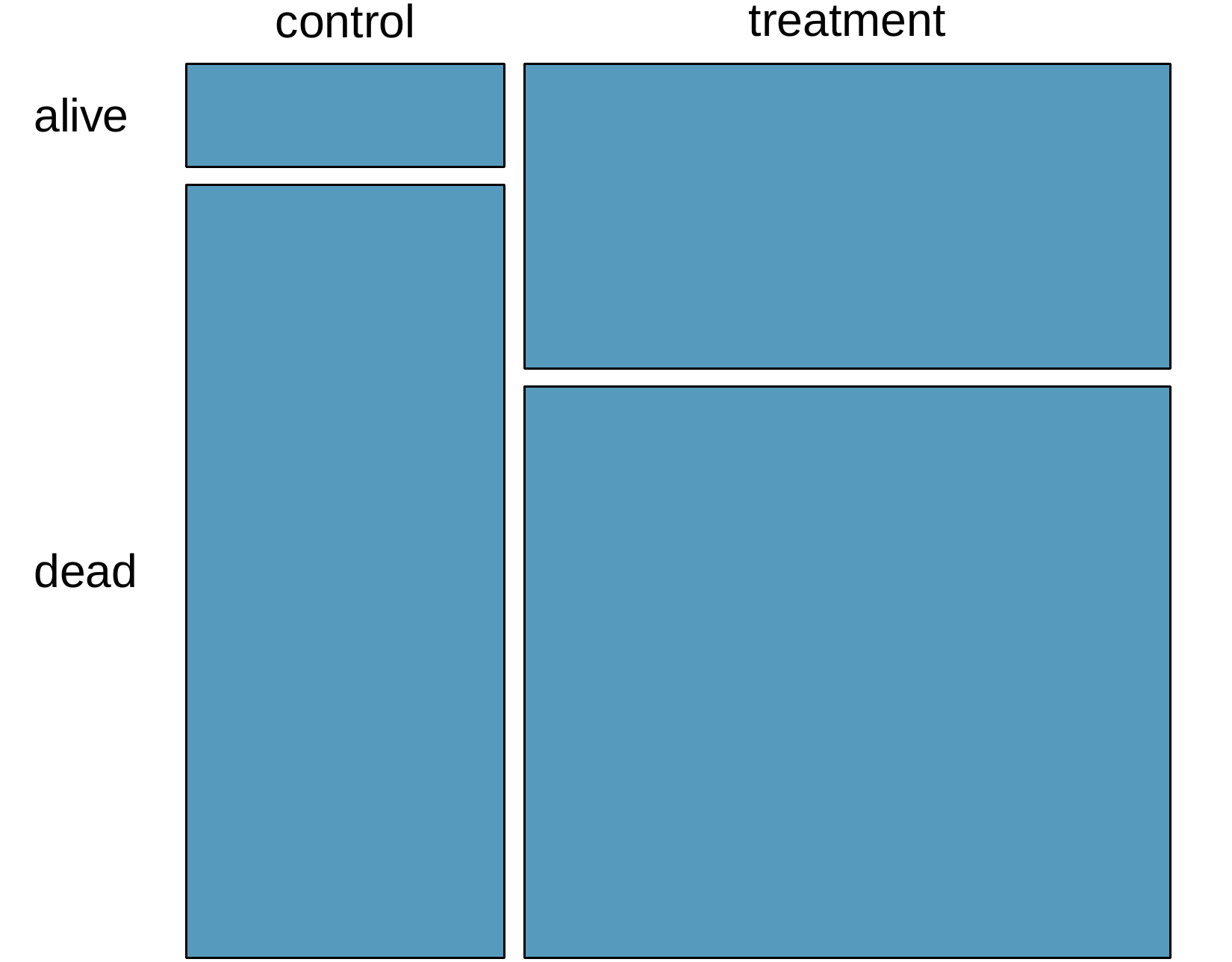
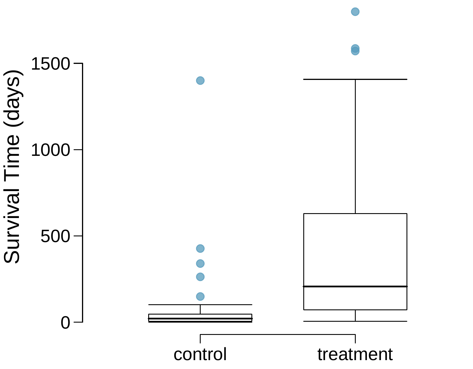
3. What do the simulation results suggest about the relationship between taking rosiglitazone and having cardiovascular problems in diabetic patients?
  🔗
  
  🔗
🔗

🔗

2. Heart transplants.

The Stanford University Heart Transplant Study was conducted to determine whether an experimental heart transplant program increased lifespan. Each patient entering the program was designated an official heart transplant candidate, meaning that he was gravely ill and would most likely benefit from a new heart. Some patients got a transplant and some did not. The variable transplant indicates which group the patients were in; patients in the treatment group got a transplant and those in the control group did not. Of the 34 patients in the control group, 30 died. Of the 69 people in the treatment group, 45 died. Another variable called survived was used to indicate whether or not the patient was alive at the end of the study.

🔗

A mosaic plot for variables "experiment group" (primary split) and "survived". The first tall rectangle for the "control" experiment group is about half the width of the second tall rectangle for "treatment". When looking at the secondary split for the control group, the "alive" outcome represents about 10% of the height and "dead" represents about 90% of the height. When looking at the secondary split for the treatment group, the "alive" outcome represents about 35% of the height and "dead" represents about 65% of the height. — (a) Mosaic plot of survival by experiment group
🔗

A side-by-side box plot is shown for the variable "Survival Time (days)" for two box plots labeled "control" and "survived". The axis for survival time spans 0 to about 1800. The box for the control group spans about 0 to 50 with the median line at about 20, and the whiskers extend down to 0 and up to about 125. There are five observations shown beyond the upper whisker at locations of about 150, 250, 300, 400, and 1400. The box for the treatment spans about 100 to 650 with the median line about 250, and the whiskers extend down to 0 and up to about 1400. There are a few points beyond the upper whiskers at about 1550, 1575, and 1800. — (a) Mosaic plot of survival by experiment group
🔗

Based on the mosaic plot, is survival independent of whether or not the patient got a transplant? Explain your reasoning.
🔗

🔗
What do the box plots below suggest about the efficacy (effectiveness) of the heart transplant treatment.
🔗

🔗
What proportion of patients in the treatment group and what proportion of patients in the control group died?
🔗

🔗
One approach for investigating whether or not the treatment is effective is to use a randomization technique.
🔗
1. What are the claims being tested?
  🔗
  
  🔗
2. The paragraph below describes the set up for such approach, if we were to do it without using statistical software. Fill in the blanks with a number or phrase, whichever is appropriate.
  🔗
  
  We write alive on \(\underline{\hspace{1cm}}\) cards representing patients who were alive at the end of the study, and dead on \(\underline{\hspace{1cm}}\) cards representing patients who were not. Then, we shuffle these cards and split them into two groups: one group of size \(\underline{\hspace{1cm}}\) representing treatment, and another group of size \(\underline{\hspace{1cm}}\) representing control. We calculate the difference between the proportion of dead cards in the treatment and control groups (treatment - control) and record this value. We repeat this 100 times to build a distribution centered at \(\underline{\hspace{1cm}}\text{.}\) Lastly, we calculate the fraction of simulations where the simulated differences in proportions are \(\underline{\hspace{1cm}}\text{.}\) If this fraction is low, we conclude that it is unlikely to have observed such an outcome by chance and that the null hypothesis should be rejected in favor of the alternative.
  🔗
  
  🔗
3. What do the simulation results shown below suggest about the effectiveness of the transplant program?
  🔗
  
  Figure 2.3.13. Simulated differences in proportions
  🔗
  
  🔗
🔗

🔗

Prev Top Next