Normal distribution

Section 4.1 Normal distribution

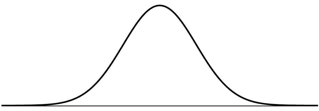
Among all the distributions we see in practice, one is overwhelmingly the most common. The symmetric, unimodal, bell curve is ubiquitous throughout statistics. Indeed it is so common, that people often know it as the normal curve or normal distribution.

🔗

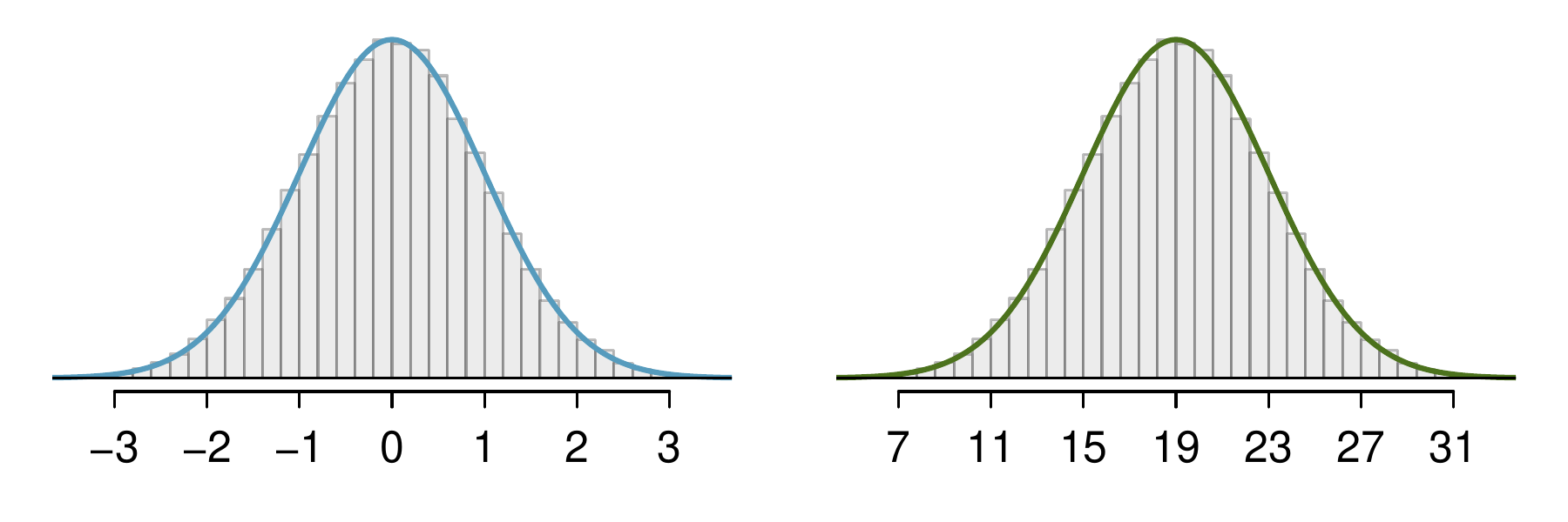
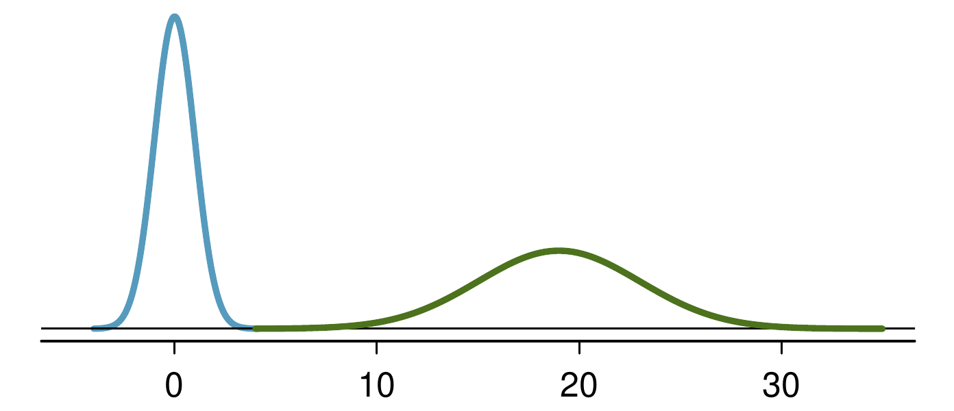
Variables such as SAT scores and heights of US adult males closely follow the normal distribution.

🔗

Subsection 4.1.1 Normal distribution model

The normal distribution always describes a symmetric, unimodal, bell-shaped curve. However, these curves can look different depending on the details of the model. Specifically, the normal distribution model can be adjusted using two parameters: mean and standard deviation. As you can probably guess, changing the mean shifts the bell curve to the left or right, while changing the standard deviation stretches or constricts the curve. Figure 4.1.2 shows the normal distribution with mean \(0\) and standard deviation \(1\) in the left panel and the normal distribution with mean \(19\) and standard deviation \(4\) in the right panel. Figure 4.1.3 shows these distributions on the same axis.

🔗

Figure 4.1.2. Both curves represent the normal distribution. However, they differ in their center and spread.
🔗

Figure 4.1.3. The normal distributions shown in Figure 4.1.2 but plotted together and on the same scale.
🔗

If a normal distribution has mean \(\mu\) and standard deviation \(\sigma\text{,}\) we may write the distribution as \(N(\mu, \sigma)\text{.}\) The two distributions in Figure 4.1.3 may be written as

\begin{gather*} N(\mu=0, \sigma=1) \quad \text{and} \quad N(\mu=19, \sigma=4) \end{gather*}

Because the mean and standard deviation describe a normal distribution exactly, they are called the distribution’s parameters.

🔗

Normal distribution facts
🔗

Many variables are nearly normal, but none are exactly normal. Thus the normal distribution, while not perfect for any single problem, is very useful for a variety of problems. We will use it in data exploration and to solve important problems in statistics.
🔗

🔗

The normal distribution with mean \(\mu = 0\) and standard deviation \(\sigma = 1\) is called the standard normal distribution.

🔗

Checkpoint 4.1.4.

Write down the short-hand for a normal distribution with (a) mean 5 and standard deviation 3, (b) mean -100 and standard deviation 10, and (c) mean 2 and standard deviation 9.

🔗

Solution.

(a) \(N(\mu=5, \sigma=3)\text{.}\) (b) \(N(\mu=-100, \sigma=10)\text{.}\) (c) \(N(\mu=2, \sigma=9)\text{.}\)

🔗

Subsection 4.1.2 Standardizing with Z-scores

We often want to put data onto a standardized scale, which can make comparisons more reasonable.

🔗

Example 4.1.5. Comparing SAT and ACT scores.

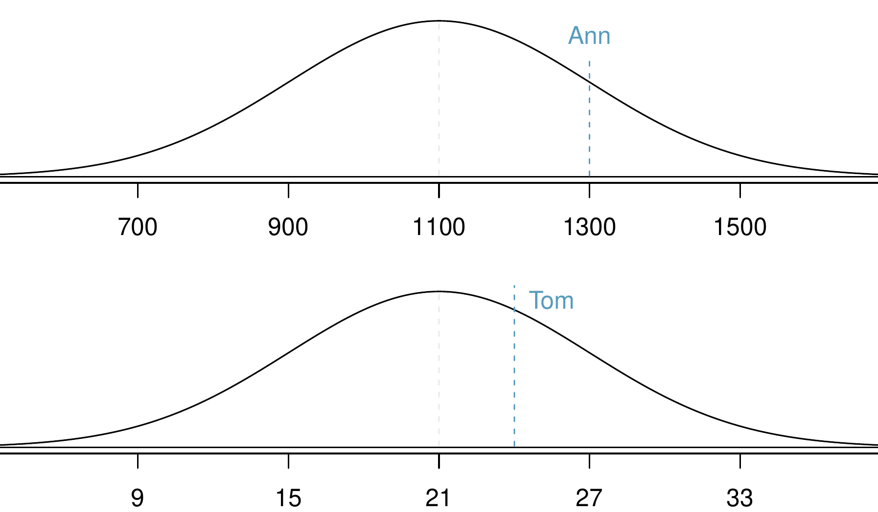
Table 4.1.6 shows the mean and standard deviation for total scores on the SAT and ACT. The distribution of SAT and ACT scores are both nearly normal. Suppose Ann scored 1300 on her SAT and Tom scored 24 on his ACT. Who performed better?

🔗

Solution.

We use the standard deviation as a guide. Ann is 1 standard deviation above average on the SAT: \(1100 + 200 = 1300\text{.}\) Tom is 0.5 standard deviations above the mean on the ACT: \(21 + 0.5 \times 6 = 24\text{.}\) In Figure 4.1.7, we can see that Ann tends to do better with respect to everyone else than Tom did, so her score was better.

🔗

Table 4.1.6. Mean and standard deviation for the SAT and ACT

🔗

	SAT	ACT
Mean	1100	21
SD	200	6

Figure 4.1.7. Ann’s and Tom’s scores shown against the SAT and ACT distributions.
🔗

Example 4.1.5 used a standardization technique called a Z-score, a method most commonly employed for nearly normal observations but that may be used with any distribution. The Z-score of an observation is defined as the number of standard deviations it falls above or below the mean. If the observation is one standard deviation above the mean, its Z-score is 1. If it is 1.5 standard deviations below the mean, then its Z-score is -1.5. If \(x\) is an observation from a distribution \(N(\mu, \sigma)\text{,}\) we define the Z-score mathematically as

\begin{equation*} Z = \frac{x - \mu}{\sigma} \end{equation*}

Using \(\mu_{SAT} = 1100\text{,}\) \(\sigma_{SAT} = 200\text{,}\) and \(x_{Ann} = 1300\text{,}\) we find Ann’s Z-score:

\begin{equation*} Z_{Ann} = \frac{x_{Ann} - \mu_{SAT}}{\sigma_{SAT}} = \frac{1300 - 1100}{200} = 1 \end{equation*}

🔗

The Z-score
🔗

The Z-score of an observation is the number of standard deviations it falls above or below the mean. We compute the Z-score for an observation \(x\) that follows a distribution with mean \(\mu\) and standard deviation \(\sigma\) using

\begin{equation*} Z = \frac{x - \mu}{\sigma} \end{equation*}

🔗

🔗

Checkpoint 4.1.8.

Use Tom’s ACT score, 24, along with the ACT mean and standard deviation to find his Z-score.

🔗

Solution.

\(Z_{Tom} = \frac{x_{Tom} - \mu_{ACT}}{\sigma_{ACT}} = \frac{24 - 21}{6} = 0.5\)

🔗

Observations above the mean always have positive Z-scores, while those below the mean always have negative Z-scores. If an observation is equal to the mean, such as an SAT score of 1100, then the Z-score is \(0\text{.}\)

🔗

Checkpoint 4.1.9.

Let \(X\) represent a random variable from \(N(\mu=3, \sigma=2)\text{,}\) and suppose we observe \(x=5.19\text{.}\) (a) Find the Z-score of \(x\text{.}\) (b) Use the Z-score to determine how many standard deviations above or below the mean \(x\) falls.

🔗

Solution.

(a) Its Z-score is given by \(Z = \frac{x-\mu}{\sigma} = \frac{5.19 - 3}{2} = \frac{2.19}{2} = 1.095\text{.}\) (b) The observation \(x\) is 1.095 standard deviations above the mean. We know it must be above the mean since \(Z\) is positive.

🔗

Checkpoint 4.1.10.

Head lengths of brushtail possums follow a normal distribution with mean 92.6 mm and standard deviation 3.6 mm. Compute the Z-scores for possums with head lengths of 95.4 mm and 85.8 mm.

🔗

Solution.

For \(x_1=95.4\) mm: \(Z_1 = \frac{x_1 - \mu}{\sigma} = \frac{95.4 - 92.6}{3.6} = 0.78\text{.}\) For \(x_2=85.8\) mm: \(Z_2 = \frac{85.8 - 92.6}{3.6} = -1.89\text{.}\)

🔗

We can use Z-scores to roughly identify which observations are more unusual than others. An observation \(x_1\) is said to be more unusual than another observation \(x_2\) if the absolute value of its Z-score is larger than the absolute value of the other observation’s Z-score: \(|Z_1| > |Z_2|\text{.}\) This technique is especially insightful when a distribution is symmetric.

🔗

Checkpoint 4.1.11.

Which of the observations in Checkpoint 4.1.10 is more unusual?

🔗

Solution.

Because the absolute value of Z-score for the second observation is larger than that of the first, the second observation has a more unusual head length.

🔗

Subsection 4.1.3 Finding tail areas

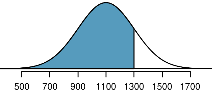
It’s very useful in statistics to be able to identify tail areas of distributions. For instance, what fraction of people have an SAT score below Ann’s score of 1300? This is the same as the percentile Ann is at, which is the percentage of cases that have lower scores than Ann. We can visualize such a tail area like the curve and shading shown in Figure 4.1.12.

🔗

Figure 4.1.12. The area to the left of \(Z\) represents the fraction of people who scored lower than Ann.
🔗

There are many techniques for doing this, and we’ll discuss three of the options.

The most common approach in practice is to use statistical software. For example, in the program R, we could find the area shown in Figure 4.1.12 using the following command, which takes in the Z-score and returns the lower tail area: pnorm(1) returns 0.8413447. According to this calculation, the region shaded that is below 1300 represents the proportion 0.841 (84.1%) of SAT test takers who had Z-scores below \(Z = 1\text{.}\) More generally, we can also specify the cutoff explicitly if we also note the mean and standard deviation: pnorm(1300, mean = 1100, sd = 200) returns 0.8413447.
🔗

There are many other software options, such as Python or SAS; even spreadsheet programs such as Excel and Google Sheets support these calculations.
🔗

🔗
A common strategy in classrooms is to use a graphing calculator, such as a TI or Casio calculator. These calculators require a series of button presses that are less concisely described. You can find instructions on using these calculators for finding tail areas of a normal distribution in the OpenIntro video library: https://www.openintro.org/videos.
🔗

🔗
The last option for finding tail areas is to use what’s called a probability table; these are occasionally used in classrooms but rarely in practice. The appendix contains such a table and a guide for how to use it.
🔗

🔗

🔗

We will solve normal distribution problems in this section by always first finding the Z-score. The reason is that we will encounter close parallels called test statistics beginning in Chapter 5; these are, in many instances, an equivalent of a Z-score.

🔗

Subsection 4.1.4 Normal probability examples

Cumulative SAT scores are approximated well by a normal model, \(N(\mu = 1100, \sigma = 200)\text{.}\)

🔗

Example 4.1.13. Finding probability of SAT score above 1190.

Shannon is a randomly selected SAT taker, and nothing is known about Shannon’s SAT aptitude. What is the probability Shannon scores at least 1190 on her SATs?

🔗

Solution.

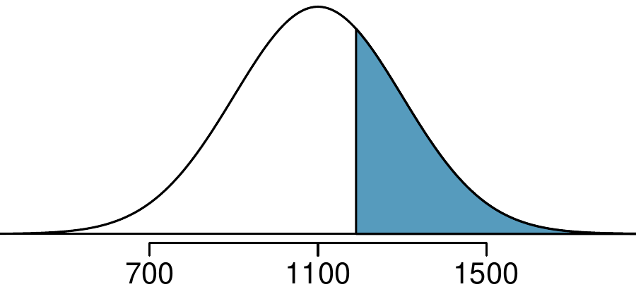
First, always draw and label a picture of the normal distribution. (Drawings need not be exact to be useful.) We are interested in the chance she scores above 1190, so we shade this upper tail:

🔗

Figure 4.1.14. Shading the upper tail above 1190
🔗

The picture shows the mean and the values at 2 standard deviations above and below the mean. The simplest way to find the shaded area under the curve makes use of the Z-score of the cutoff value. With \(\mu = 1100\text{,}\) \(\sigma = 200\text{,}\) and the cutoff value \(x = 1190\text{,}\) the Z-score is computed as

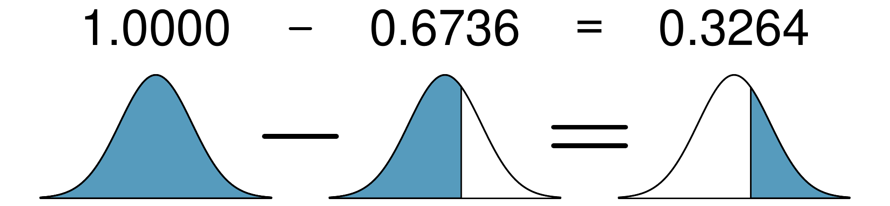
\begin{equation*} Z = \frac{x - \mu}{\sigma} = \frac{1190 - 1100}{200} = \frac{90}{200} = 0.45 \end{equation*}

Using statistical software (or another preferred method), we can find the area left of \(Z = 0.45\) as 0.6736. To find the area above \(Z = 0.45\text{,}\) we compute one minus the area of the lower tail:

🔗

Figure 4.1.15. Computing the upper tail area
🔗

The probability Shannon scores at least 1190 on the SAT is 0.3264.

🔗

Always draw a picture first, and find the Z-score second
🔗

For any normal probability situation, always always always draw and label the normal curve and shade the area of interest first. The picture will provide an estimate of the probability. After drawing a figure to represent the situation, identify the Z-score for the value of interest.
🔗

🔗

Checkpoint 4.1.16.

If the probability of Shannon scoring at least 1190 is 0.3264, then what is the probability she scores less than 1190? Draw the normal curve representing this exercise, shading the lower region instead of the upper one.

🔗

Solution.

We found this probability in Example 4.1.13: 0.6736.

🔗

Example 4.1.17. Finding a percentile.

Edward earned a 1030 on his SAT. What is his percentile?

🔗

Solution.

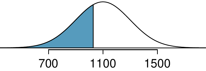
First, a picture is needed. Edward’s percentile is the proportion of people who do not get as high as a 1030. These are the scores to the left of 1030.

🔗

Figure 4.1.18. Shading the lower tail below 1030
🔗

Identifying the mean \(\mu=1100\text{,}\) the standard deviation \(\sigma=200\text{,}\) and the cutoff for the tail area \(x=1030\) makes it easy to compute the Z-score:

\begin{equation*} Z = \frac{x - \mu}{\sigma} = \frac{1030 - 1100}{200} = -0.35 \end{equation*}

Using statistical software, we get a tail area of 0.3632. Edward is at the 36\(^{th}\) percentile.

🔗

Checkpoint 4.1.19.

Use the results of Example 4.1.17 to compute the proportion of SAT takers who did better than Edward. Also draw a new picture.

🔗

Solution.

If Edward did better than 36% of SAT takers, then about 64% must have done better than him.

🔗

Finding areas to the right
🔗

Many software programs return the area to the left when given a Z-score. If you would like the area to the right, first find the area to the left and then subtract this amount from one.
🔗

🔗

Checkpoint 4.1.20.

Stuart earned an SAT score of 1500. Draw a picture for each part. (a) What is his percentile? (b) What percent of SAT takers did better than Stuart?

🔗

Solution.

We leave the drawings to you. (a) \(Z = \frac{1500 - 1100}{200} = 2 \to 0.9772\text{.}\) (b) \(1 - 0.9772 = 0.0228\text{.}\)

🔗

Based on a sample of 100 men, the heights of male adults in the US is nearly normal with mean 70.0’’ and standard deviation 3.3’’.

🔗

Checkpoint 4.1.21.

Mike is 5’7’’ and Jose is 6’4’’, and they both live in the US. (a) What is Mike’s height percentile? (b) What is Jose’s height percentile? Also draw one picture for each part.

🔗

Solution.

First put the heights into inches: 67 and 76 inches. (a) \(Z_{Mike} = \frac{67 - 70}{3.3} = -0.91 \to 0.1814\text{.}\) (b) \(Z_{Jose} = \frac{76 - 70}{3.3} = 1.82 \to 0.9656\text{.}\)

🔗

The last several problems have focused on finding the percentile (lower tail) or the upper tail for a particular observation. What if you would like to know the observation corresponding to a particular percentile?

🔗

Example 4.1.22. Finding height at 40th percentile.

Erik’s height is at the 40\(^{th}\) percentile. How tall is he?

🔗

Solution.

As always, first draw the picture.

🔗

Figure 4.1.23. Finding the height at the 40th percentile
🔗

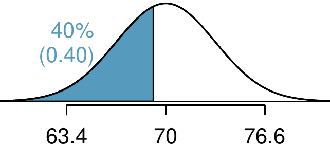
In this case, the lower tail probability is known (0.40), which can be shaded on the diagram. We want to find the observation that corresponds to this value. As a first step in this direction, we determine the Z-score associated with the 40\(^{th}\) percentile. Using software, we can obtain the corresponding Z-score of about -0.25.

🔗

Knowing \(Z_{Erik} = -0.25\) and the population parameters \(\mu = 70\) and \(\sigma = 3.3\) inches, the Z-score formula can be set up to determine Erik’s unknown height, labeled \(x_{Erik}\text{:}\)

\begin{equation*} -0.25 = Z_{Erik} = \frac{x_{Erik} - \mu}{\sigma} = \frac{x_{Erik} - 70}{3.3} \end{equation*}

Solving for \(x_{Erik}\) yields a height of 69.18 inches. That is, Erik is about 5’9’’.

🔗

Example 4.1.24. Finding height at 82nd percentile.

What is the adult male height at the 82\(^{nd}\) percentile?

🔗

Solution.

Again, we draw the figure first.

🔗

Figure 4.1.25. Finding the height at the 82nd percentile
🔗

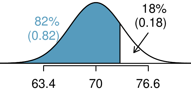
Next, we want to find the Z-score at the 82\(^{nd}\) percentile, which will be a positive value and can be found using software as \(Z = 0.92\text{.}\) Finally, the height \(x\) is found using the Z-score formula with the known mean \(\mu\text{,}\) standard deviation \(\sigma\text{,}\) and Z-score \(Z = 0.92\text{:}\)

\begin{equation*} 0.92 = Z = \frac{x-\mu}{\sigma} = \frac{x - 70}{3.3} \end{equation*}

This yields 73.04 inches or about 6’1’’ as the height at the 82\(^{nd}\) percentile.

🔗

Checkpoint 4.1.26.

The SAT scores follow \(N(1100, 200)\text{.}\) (a) What is the 95\(^{th}\) percentile for SAT scores? (b) What is the 97.5\(^{th}\) percentile for SAT scores?

🔗

Solution.

Short answers: (a) \(Z_{95} = 1.6449 \to 1429\) SAT score. (b) \(Z_{97.5} = 1.96 \to 1492\) SAT score.

🔗

Checkpoint 4.1.27.

Adult male heights follow \(N(70.0'', 3.3'')\text{.}\) (a) What is the probability that a randomly selected male adult is at least 6’2’’ (74 inches)? (b) What is the probability that a male adult is shorter than 5’9’’ (69 inches)?

🔗

Solution.

Short answers: (a) \(Z = 1.21 \to 0.8869\text{,}\) then subtract this value from 1 to get 0.1131. (b) \(Z = -0.30 \to 0.3821\text{.}\)

🔗

Example 4.1.28. Finding probability between two values.

What is the probability that a random adult male is between 5’9’’ and 6’2’’?

🔗

Solution.

These heights correspond to 69 inches and 74 inches. First, draw the figure. The area of interest is no longer an upper or lower tail.

🔗

Figure 4.1.29. Finding area between two values
🔗

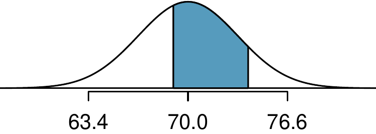
The total area under the curve is 1. If we find the area of the two tails that are not shaded (from Checkpoint 4.1.27, these areas are 0.3821 and 0.1131), then we can find the middle area:

🔗

Figure 4.1.30. Subtracting the tail areas from 1
🔗

That is, the probability of being between 5’9’’ and 6’2’’ is 0.5048.

🔗

Checkpoint 4.1.31.

SAT scores follow \(N(1100, 200)\text{.}\) What percent of SAT takers get between 1100 and 1400?

🔗

Solution.

This is an abbreviated solution. (Be sure to draw a figure!) First find the percent who get below 1100 and the percent that get above 1400: \(Z_{1100} = 0.00 \to 0.5000\) (area below), \(Z_{1400} = 1.5 \to 0.0668\) (area above). Final answer: \(1.0000 - 0.5000 - 0.0668 = 0.4332\text{.}\)

🔗

Checkpoint 4.1.32.

Adult male heights follow \(N(70.0'', 3.3'')\text{.}\) What percent of adult males are between 5’5’’ and 5’7’’?

🔗

Solution.

5’5’’ is 65 inches (\(Z = -1.52\)). 5’7’’ is 67 inches (\(Z = -0.91\)). Numerical solution: \(1.000 - 0.0643 - 0.8186 = 0.1171\text{,}\) i.e. 11.71%.

🔗

Subsection 4.1.5 68-95-99.7 rule

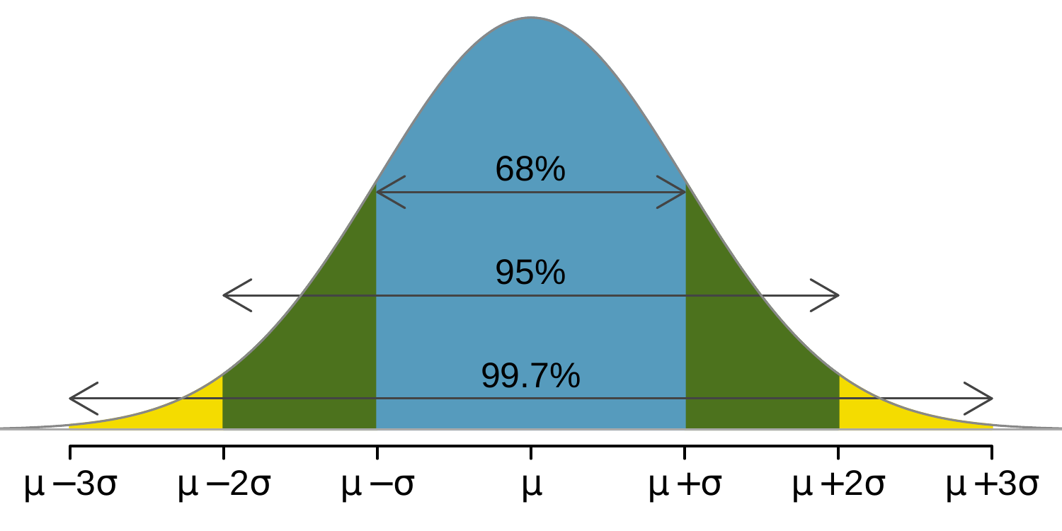
Here, we present a useful rule of thumb for the probability of falling within 1, 2, and 3 standard deviations of the mean in the normal distribution. This will be useful in a wide range of practical settings, especially when trying to make a quick estimate without a calculator or Z-table.

🔗

Figure 4.1.33. Probabilities for falling within 1, 2, and 3 standard deviations of the mean in a normal distribution.
🔗

Checkpoint 4.1.34.

Use software, a calculator, or a probability table to confirm that about 68%, 95%, and 99.7% of observations fall within 1, 2, and 3 standard deviations of the mean in the normal distribution, respectively. For instance, first find the area that falls between \(Z=-1\) and \(Z=1\text{,}\) which should have an area of about 0.68. Similarly there should be an area of about 0.95 between \(Z=-2\) and \(Z=2\text{.}\)

🔗

Solution.

First draw the pictures. Using software, we get 0.6827 within 1 standard deviation, 0.9545 within 2 standard deviations, and 0.9973 within 3 standard deviations.

🔗

It is possible for a normal random variable to fall 4, 5, or even more standard deviations from the mean. However, these occurrences are very rare if the data are nearly normal. The probability of being further than 4 standard deviations from the mean is about 1-in-15,000. For 5 and 6 standard deviations, it is about 1-in-2 million and 1-in-500 million, respectively.

🔗

Checkpoint 4.1.35.

SAT scores closely follow the normal model with mean \(\mu = 1100\) and standard deviation \(\sigma = 200\text{.}\) (a) About what percent of test takers score 700 to 1500? (b) What percent score between 1100 and 1500?

🔗

Solution.

(a) 700 and 1500 represent two standard deviations below and above the mean, which means about 95% of test takers will score between 700 and 1500. (b) We found that 700 to 1500 represents about 95% of test takers. These test takers would be evenly split by the center of the distribution, 1100, so \(\frac{95\%}{2} = 47.5\%\) of all test takers score between 1100 and 1500.

🔗

Exercises 4.1.6 Exercises

1. Area under the curve, Part I.

What percent of a standard normal distribution \(N(\mu=0, \sigma=1)\) is found in each region? Be sure to draw a graph.

🔗

\(\displaystyle Z \lt -1.35\)
🔗

🔗
\(\displaystyle Z > 1.48\)
🔗

🔗
\(\displaystyle -0.4 \lt Z \lt 1.5\)
🔗

🔗
\(\displaystyle |Z| > 2\)
🔗

🔗

🔗

2. Area under the curve, Part II.

What percent of a standard normal distribution \(N(\mu=0, \sigma=1)\) is found in each region? Be sure to draw a graph.

🔗

\(\displaystyle Z > -1.13\)
🔗

🔗
\(\displaystyle Z \lt 0.18\)
🔗

🔗
\(\displaystyle Z > 8\)
🔗

🔗
\(\displaystyle |Z| \lt 0.5\)
🔗

🔗

🔗

3. GRE scores, Part I.

Sophia who took the Graduate Record Examination (GRE) scored 160 on the Verbal Reasoning section and 157 on the Quantitative Reasoning section. The mean score for Verbal Reasoning section for all test takers was 151 with a standard deviation of 7, and the mean score for the Quantitative Reasoning was 153 with a standard deviation of 7.67. Suppose that both distributions are nearly normal.

🔗

Write down the short-hand for these two normal distributions.
🔗

🔗
What is Sophia’s Z-score on the Verbal Reasoning section? On the Quantitative Reasoning section? Draw a standard normal distribution curve and mark these two Z-scores.
🔗

🔗
What do these Z-scores tell you?
🔗

🔗
Relative to others, which section did she do better on?
🔗

🔗
Find her percentile scores for the two exams.
🔗

🔗
What percent of the test takers did better than her on the Verbal Reasoning section? On the Quantitative Reasoning section?
🔗

🔗
Explain why simply comparing raw scores from the two sections could lead to an incorrect conclusion as to which section a student did better on.
🔗

🔗
If the distributions of the scores on these exams are not nearly normal, would your answers to parts (b) - (f) change? Explain your reasoning.
🔗

🔗

🔗

4. Triathlon times, Part I.

In triathlons, it is common for racers to be placed into age and gender groups. Friends Leo and Mary both completed the Hermosa Beach Triathlon, where Leo competed in the Men, Ages 30 - 34 group while Mary competed in the Women, Ages 25 - 29 group. Leo completed the race in 1:22:28 (4948 seconds), while Mary completed the race in 1:31:53 (5513 seconds). Obviously Leo finished faster, but they are curious about how they did within their respective groups. Can you help them? Here is some information on the performance of their groups:

🔗

The finishing times of the Men, Ages 30 - 34 group has a mean of 4313 seconds with a standard deviation of 583 seconds.
🔗

🔗
The finishing times of the Women, Ages 25 - 29 group has a mean of 5261 seconds with a standard deviation of 807 seconds.
🔗

🔗
The distributions of finishing times for both groups are approximately normal.
🔗

🔗

🔗

Remember: a better performance corresponds to a faster finish.

🔗

Write down the short-hand for these two normal distributions.
🔗

🔗
What are the Z-scores for Leo’s and Mary’s finishing times? What do these Z-scores tell you?
🔗

🔗
Did Leo or Mary rank better in their respective groups? Explain your reasoning.
🔗

🔗
What percent of the triathletes did Leo finish faster than in his group?
🔗

🔗
What percent of the triathletes did Mary finish faster than in her group?
🔗

🔗
If the distributions of finishing times are not nearly normal, would your answers to parts (b)-(e) change? Explain your reasoning.
🔗

🔗

🔗

5. GRE scores, Part II.

In Exercise 4.1.6.3 we saw two distributions for GRE scores: \(N(\mu=151, \sigma=7)\) for the verbal part of the exam and \(N(\mu=153, \sigma=7.67)\) for the quantitative part. Use this information to compute each of the following:

🔗

The score of a student who scored in the 80\(^{th}\) percentile on the Quantitative Reasoning section.
🔗

🔗
The score of a student who scored worse than 70% of the test takers in the Verbal Reasoning section.
🔗

🔗

🔗

6. Triathlon times, Part II.

In Exercise 4.1.6.4 we saw two distributions for triathlon times: \(N(\mu=4313, \sigma=583)\) for Men, Ages 30 - 34 and \(N(\mu=5261, \sigma=807)\) for the Women, Ages 25 - 29 group. Times are listed in seconds. Use this information to compute each of the following:

🔗

The cutoff time for the fastest 5% of athletes in the men’s group, i.e. those who took the shortest 5% of time to finish.
🔗

🔗
The cutoff time for the slowest 10% of athletes in the women’s group.
🔗

🔗

🔗

7. LA weather, Part I.

The average daily high temperature in June in LA is 77°F with a standard deviation of 5°F. Suppose that the temperatures in June closely follow a normal distribution.

🔗

What is the probability of observing an 83°F temperature or higher in LA during a randomly chosen day in June?
🔗

🔗
How cool are the coldest 10% of the days (days with lowest high temperature) during June in LA?
🔗

🔗

🔗

8. CAPM.

The Capital Asset Pricing Model (CAPM) is a financial model that assumes returns on a portfolio are normally distributed. Suppose a portfolio has an average annual return of 14.7% (i.e. an average gain of 14.7%) with a standard deviation of 33%. A return of 0% means the value of the portfolio doesn’t change, a negative return means that the portfolio loses money, and a positive return means that the portfolio gains money.

🔗

What percent of years does this portfolio lose money, i.e. have a return less than 0%?
🔗

🔗
What is the cutoff for the highest 15% of annual returns with this portfolio?
🔗

🔗

🔗

9. LA weather, Part II.

Exercise 4.1.6.7 states that average daily high temperature in June in LA is 77°F with a standard deviation of 5°F, and it can be assumed that they follow a normal distribution. We use the following equation to convert °F (Fahrenheit) to °C (Celsius):

\begin{equation*} C = (F - 32) \times \frac{5}{9} \end{equation*}

🔗

Write the probability model for the distribution of temperature in °C in June in LA.
🔗

🔗
What is the probability of observing a 28°C (which roughly corresponds to 83°F) temperature or higher in June in LA? Calculate using the °C model from part (a).
🔗

🔗
Did you get the same answer or different answers in part (b) of this question and part (a) of Exercise 4.1.6.7? Are you surprised? Explain.
🔗

🔗
Estimate the IQR of the temperatures (in °C) in June in LA.
🔗

🔗

🔗

10. Find the SD.

Cholesterol levels for women aged 20 to 34 follow an approximately normal distribution with mean 185 milligrams per deciliter (mg/dl). Women with cholesterol levels above 220 mg/dl are considered to have high cholesterol and about 18.5% of women fall into this category. What is the standard deviation of the distribution of cholesterol levels for women aged 20 to 34?

🔗

Prev Top Next