Point Estimates and Sampling Variability

Section 5.1 Point Estimates and Sampling Variability

Companies such as Pew Research frequently conduct polls as a way to understand the state of public opinion or knowledge on many topics, including politics, scientific understanding, brand recognition, and more. The ultimate goal in taking a poll is generally to use the responses to estimate the opinion or knowledge of the broader population.

🔗

Subsection 5.1.1 Point Estimates and Error

Suppose a poll suggested the US President’s approval rating is 45%. We would consider 45% to be a point estimate of the approval rating we might see if we collected responses from the entire population. This entire-population response proportion is generally referred to as the parameter of interest.

🔗

When the parameter is a proportion, it is often denoted by $p\text{,}$ and we often refer to the sample proportion as $\hat{p}$ (pronounced p-hat

Not to be confused with phat, the slang term used for something cool, like this book.

). Unless we collect responses from every individual in the population, $p$ remains unknown, and we use $\hat{p}$ as our estimate of $p\text{.}$ The difference we observe from the poll versus the parameter is called the error in the estimate.

🔗

Generally, the error consists of two aspects: sampling error and bias.

🔗

Sampling error, sometimes called sampling uncertainty, describes how much an estimate will tend to vary from one sample to the next. For instance, the estimate from one sample might be 1% too low while in another it may be 3% too high. Much of statistics, including much of this book, is focused on understanding and quantifying sampling error, and we will find it useful to consider a sample’s size to help us quantify this error; the sample size is often represented by the letter $n\text{.}$

🔗

Bias describes a systematic tendency to over- or under-estimate the true population value. For example, if we were taking a student poll asking about support for a new college stadium, we’d probably get a biased estimate of the stadium’s level of student support by wording the question as, Do you support your school by supporting funding for the new stadium? We try to minimize bias through thoughtful data collection procedures, which were discussed in Chapter 1 and are the topic of many other books.

🔗

Subsection 5.1.2 Understanding the Variability of a Point Estimate

Suppose the proportion of American adults who support the expansion of solar energy is $p = 0.88\text{,}$ which is our parameter of interest.

We haven’t actually conducted a census to measure this value perfectly. However, a very large sample has suggested the actual level of support is about 88%.

If we were to take a poll of 1000 American adults on this topic, the estimate would not be perfect, but how close might we expect the sample proportion in the poll would be to 88%? We want to understand, how does the sample proportion $\hat{p}$ behave when the true population proportion is 0.88.

88% written as a proportion would be 0.88. It is common to switch between proportion and percent. However, formulas presented in this book always refer to the proportion, not the percent.

Let’s find out!

🔗

We can simulate responses we would get from a simple random sample of 1000 American adults, which is only possible because we know the actual support for expanding solar energy is 0.88. Here’s how we might go about constructing such a simulation:

🔗

There were about 250 million American adults in 2018. On 250 million pieces of paper, write “support” on 88% of them and “not” on the other 12%.

🔗
Mix up the pieces of paper and pull out 1000 pieces to represent our sample of 1000 American adults.

🔗
Compute the fraction of the sample that say “support”.

🔗

Any volunteers to conduct this simulation? Probably not. Running this simulation with 250 million pieces of paper would be time-consuming and very costly, but we can simulate it using computer code; we’ve written a short program in Figure 5.1.1 in case you are curious what the computer code looks like. In this simulation, the sample gave a point estimate of $\hat{p}_1 = 0.894\text{.}$ We know the population proportion for the simulation was $p = 0.88\text{,}$ so we know the estimate had an error of $0.894 - 0.88 = +0.014\text{.}$

🔗

# 1. Create a set of 250 million entries,
#    where 88% of them are "support" and 12% are "not".
pop_size <- 250000000
possible_entries <- c(rep("support", 0.88 * pop_size),
                       rep("not", 0.12 * pop_size))

# 2. Sample 1000 entries without replacement.
sampled_entries <- sample(possible_entries, size = 1000)

# 3. Compute p-hat: count the number that are "support",
#    then divide by the sample size.
sum(sampled_entries == "support") / 1000

Figure 5.1.1. For those curious, this is code for a single $\hat{p}$ simulation using the statistical software called R. Each line that starts with # is a code comment, which is used to describe in regular language what the code is doing. OpenIntro has provided software labs in R at openintro.org/book/os for anyone interested in learning more.

🔗

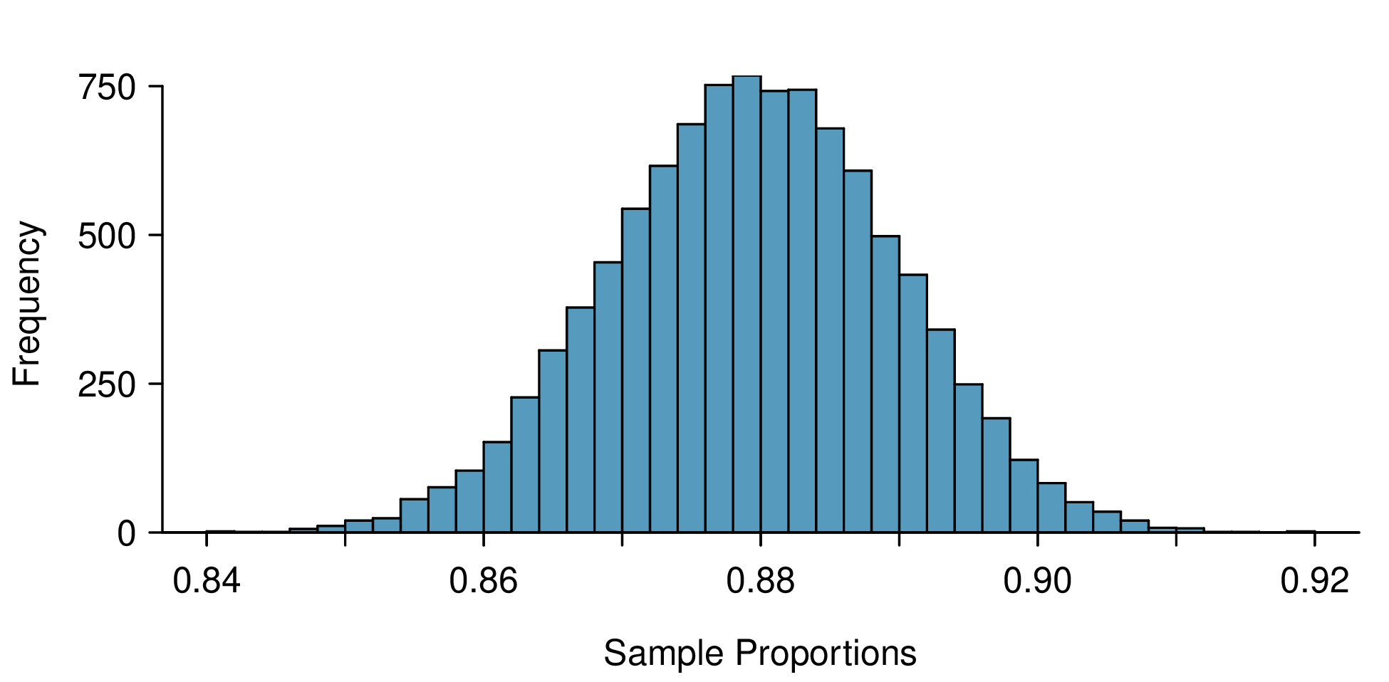
One simulation isn’t enough to get a great sense of the distribution of estimates we might expect in the simulation, so we should run more simulations. In a second simulation, we get $\hat{p}_2 = 0.885\text{,}$ which has an error of +0.005. In another, $\hat{p}_3 = 0.878$ for an error of -0.002. And in another, an estimate of $\hat{p}_4 = 0.859$ with an error of -0.021. With the help of a computer, we’ve run the simulation 10,000 times and created a histogram of the results from all 10,000 simulations in Figure 5.1.2. This distribution of sample proportions is called a sampling distribution. We can characterize this sampling distribution as follows:

🔗

Center. The center of the distribution is $\bar{x}_{\hat{p}} = 0.880\text{,}$ which is the same as the parameter. Notice that the simulation mimicked a simple random sample of the population, which is a straightforward sampling strategy that helps avoid sampling bias.

🔗
Spread. The standard deviation of the distribution is $s_{\hat{p}} = 0.010\text{.}$ When we’re talking about a sampling distribution or the variability of a point estimate, we typically use the term standard error rather than standard deviation, and the notation $SE_{\hat{p}}$ is used for the standard error associated with the sample proportion.

🔗
Shape. The distribution is symmetric and bell-shaped, and it resembles a normal distribution.

🔗

These findings are encouraging! When the population proportion is $p = 0.88$ and the sample size is $n = 1000\text{,}$ the sample proportion $\hat{p}$ tends to give a pretty good estimate of the population proportion. We also have the interesting observation that the histogram resembles a normal distribution.

🔗

A histogram is shown for 10,000 sample proportions where each sample is taken from a population where the population proportion is 0.88 and the sample size is n = 1000. The distribution is bell-shaped (appears nearly normal), is centered at 0.88 and has a standard deviation of about 0.01. — Figure 5.1.2. A histogram of 10,000 sample proportions, where each sample is taken from a population where the population proportion is 0.88 and the sample size is $n = 1000\text{.}$
🔗

Sampling distributions are never observed, but we keep them in mind.

In real-world applications, we never actually observe the sampling distribution, yet it is useful to always think of a point estimate as coming from such a hypothetical distribution. Understanding the sampling distribution will help us characterize and make sense of the point estimates that we do observe.

🔗

Example 5.1.3.

If we used a much smaller sample size of $n = 50\text{,}$ would you guess that the standard error for $\hat{p}$ would be larger or smaller than when we used $n = 1000\text{?}$

🔗

Solution.

Intuitively, it seems like more data is better than less data, and generally that is correct! The typical error when $p = 0.88$ and $n = 50$ would be larger than the error we would expect when $n = 1000\text{.}$

🔗

Example 5.1.3 highlights an important property we will see again and again: a bigger sample tends to provide a more precise point estimate than a smaller sample.

🔗

Subsection 5.1.3 Central Limit Theorem

The distribution in Figure 5.1.2 looks an awful lot like a normal distribution. That is no anomaly; it is the result of a general principle called the Central Limit Theorem.

🔗

Central Limit Theorem and the success-failure condition.

When observations are independent and the sample size is sufficiently large, the sample proportion $\hat{p}$ will tend to follow a normal distribution with the following mean and standard error:

🔗

In order for the Central Limit Theorem to hold, the sample size is typically considered sufficiently large when $np \geq 10$ and $n(1-p) \geq 10\text{,}$ which is called the success-failure condition.

🔗

The Central Limit Theorem is incredibly important, and it provides a foundation for much of statistics. As we begin applying the Central Limit Theorem, be mindful of the two technical conditions: the observations must be independent, and the sample size must be sufficiently large such that $np \geq 10$ and $n(1-p) \geq 10\text{.}$

🔗

Example 5.1.4.

Earlier we estimated the mean and standard error of $\hat{p}$ using simulated data when $p = 0.88$ and $n = 1000\text{.}$ Confirm that the Central Limit Theorem applies and the sampling distribution is approximately normal.

🔗

Solution.

Independence. There are $n = 1000$ observations for each sample proportion $\hat{p}\text{,}$ and each of those observations are independent draws. The most common way for observations to be considered independent is if they are from a simple random sample.
🔗

🔗
Success-failure condition. We can confirm the sample size is sufficiently large by checking the success-failure condition and confirming the two calculated values are greater than 10:

\begin{align*} np \amp= 1000 \times 0.88 = 880 \geq 10\\ n(1-p) \amp= 1000 \times (1 - 0.88) = 120 \geq 10 \end{align*}

🔗

🔗

The independence and success-failure conditions are both satisfied, so the Central Limit Theorem applies, and it’s reasonable to model $\hat{p}$ using a normal distribution.

🔗

How to verify sample observations are independent.

Subjects in an experiment are considered independent if they undergo random assignment to the treatment groups.

🔗

If the observations are from a simple random sample, then they are independent.

🔗

If a sample is from a seemingly random process, e.g. an occasional error on an assembly line, checking independence is more difficult. In this case, use your best judgement.

🔗

An additional condition that is sometimes added for samples from a population is that they are no larger than 10% of the population. When the sample exceeds 10% of the population size, the methods we discuss tend to overestimate the sampling error slightly versus what we would get using more advanced methods.

⁴

For example, we could use what’s called the finite population correction factor: if the sample is of size $n$ and the population size is $N\text{,}$ then we can multiply the typical standard error formula by $\sqrt{\frac{N-n}{N-1}}$ to obtain a smaller, more precise estimate of the actual standard error. When $n < 0.1 \times N\text{,}$ this correction factor is relatively small.

This is very rarely an issue, and when it is an issue, our methods tend to be conservative, so we consider this additional check as optional.

🔗

Example 5.1.5.

Compute the theoretical mean and standard error of $\hat{p}$ when $p = 0.88$ and $n = 1000\text{,}$ according to the Central Limit Theorem.

🔗

Solution.

The mean of the $\hat{p}$’s is simply the population proportion:

\begin{equation*} \mu_{\hat{p}} = 0.88 \end{equation*}

🔗

The calculation of the standard error of $\hat{p}$ uses the following formula:

\begin{align*} SE_{\hat{p}} \amp= \sqrt{\frac{p(1-p)}{n}}\\ \amp= \sqrt{\frac{0.88 \times (1 - 0.88)}{1000}}\\ \amp= 0.010 \end{align*}

🔗

Example 5.1.6.

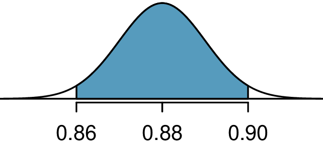
Estimate how frequently the sample proportion $\hat{p}$ should be within 0.02 (2%) of the population value, $p = 0.88\text{.}$ Based on Example 5.1.4 and Example 5.1.5, we know that the distribution is approximately $N(\mu_{\hat{p}} = 0.88, SE_{\hat{p}} = 0.010)\text{.}$

🔗

Solution.

After so much practice in Section 4.1, this normal distribution example will hopefully feel familiar! We would like to understand the fraction of $\hat{p}$’s between 0.86 and 0.90:

🔗

Normal curve centered at 0.88 with shaded region between 0.86 and 0.90 — Figure 5.1.7. A normal distribution centered at 0.88 with a standard deviation of 0.01 is shown, where the region between 0.86 and 0.90 has been shaded.
🔗

With $\mu_{\hat{p}} = 0.88$ and $SE_{\hat{p}} = 0.010\text{,}$ we can compute the Z-score for both the left and right cutoffs:

\begin{align*} Z_{0.86} \amp= \frac{0.86 - 0.88}{0.010} = -2\\ Z_{0.90} \amp= \frac{0.90 - 0.88}{0.010} = 2 \end{align*}

🔗

We can use either statistical software, a graphing calculator, or a table to find the areas to the tails, and in any case we will find that they are each 0.0228. The total tail areas are $2 \times 0.0228 = 0.0456\text{,}$ which leaves the shaded area of 0.9544. That is, about 95.44% of the sampling distribution in Figure 5.1.2 is within $\pm 0.02$ of the population proportion, $p = 0.88\text{.}$

🔗

Checkpoint 5.1.8.

In Example 5.1.3 we discussed how a smaller sample would tend to produce a less reliable estimate. Explain how this intuition is reflected in the formula for $SE_{\hat{p}} = \sqrt{\frac{p(1-p)}{n}}\text{.}$

⁵

Since the sample size $n$ is in the denominator (on the bottom) of the fraction, a bigger sample size means the entire expression when calculated will tend to be smaller. That is, a larger sample size would correspond to a smaller standard error.

🔗

Subsection 5.1.4 Applying the Central Limit Theorem to a real-world setting

We do not actually know the population proportion unless we conduct an expensive poll of all individuals in the population. Our earlier value of $p = 0.88$ was based on poll conducted by Pew Research of 1000 American adults that found $\hat{p} = 0.887$ of them favored expanding solar energy. The researchers might have wondered: does the sample proportion from the poll approximately follow a normal distribution? We can check the conditions from the Central Limit Theorem:

🔗

Independence. The poll is a simple random sample of American adults, which means that the observations are independent.
🔗

🔗
Success-failure condition. To check this condition, we need the population proportion, $p\text{,}$ to check if both $np$ and $n(1-p)$ are greater than 10. However, we do not actually know $p\text{,}$ which is exactly why the pollsters would take a sample! In cases like these, we often use $\hat{p}$ as our next best way to check the success-failure condition:

\begin{align*} n\hat{p} \amp= 1000 \times 0.887 = 887\\ n(1-\hat{p}) \amp= 1000 \times (1 - 0.887) = 113 \end{align*}

The sample proportion $\hat{p}$ acts as a reasonable substitute for $p$ during this check, and each value in this case is well above the minimum of 10.

🔗

🔗

This substitution approximation of using $\hat{p}$ in place of $p$ is also useful when computing the standard error of the sample proportion:

\begin{align*} SE_{\hat{p}} \amp= \sqrt{\frac{p(1-p)}{n}}\\ \amp\approx \sqrt{\frac{\hat{p}(1-\hat{p})}{n}}\\ \amp= \sqrt{\frac{0.887 \times (1 - 0.887)}{1000}}\\ \amp= 0.010 \end{align*}

This substitution technique is sometimes referred to as the “plug-in principle”. In this case, $SE_{\hat{p}}$ didn’t change enough to be detected using only 3 decimal places versus when we completed the calculation with 0.88 earlier. The computed standard error tends to be reasonably stable even when observing slightly different proportions in one sample or another.

🔗

Subsection 5.1.5 More details regarding the Central Limit Theorem

We’ve applied the Central Limit Theorem in numerous examples so far this chapter:

🔗

When observations are independent and the sample size is sufficiently large, the distribution of $\hat{p}$ resembles a normal distribution with

\begin{align*} \mu_{\hat{p}} \amp= p\\ SE_{\hat{p}} \amp= \sqrt{\frac{p(1-p)}{n}} \end{align*}

The sample size is considered sufficiently large when $np \geq 10$ and $n(1-p) \geq 10\text{.}$

🔗

🔗

In this section, we’ll explore the success-failure condition and seek to better understand the Central Limit Theorem.

🔗

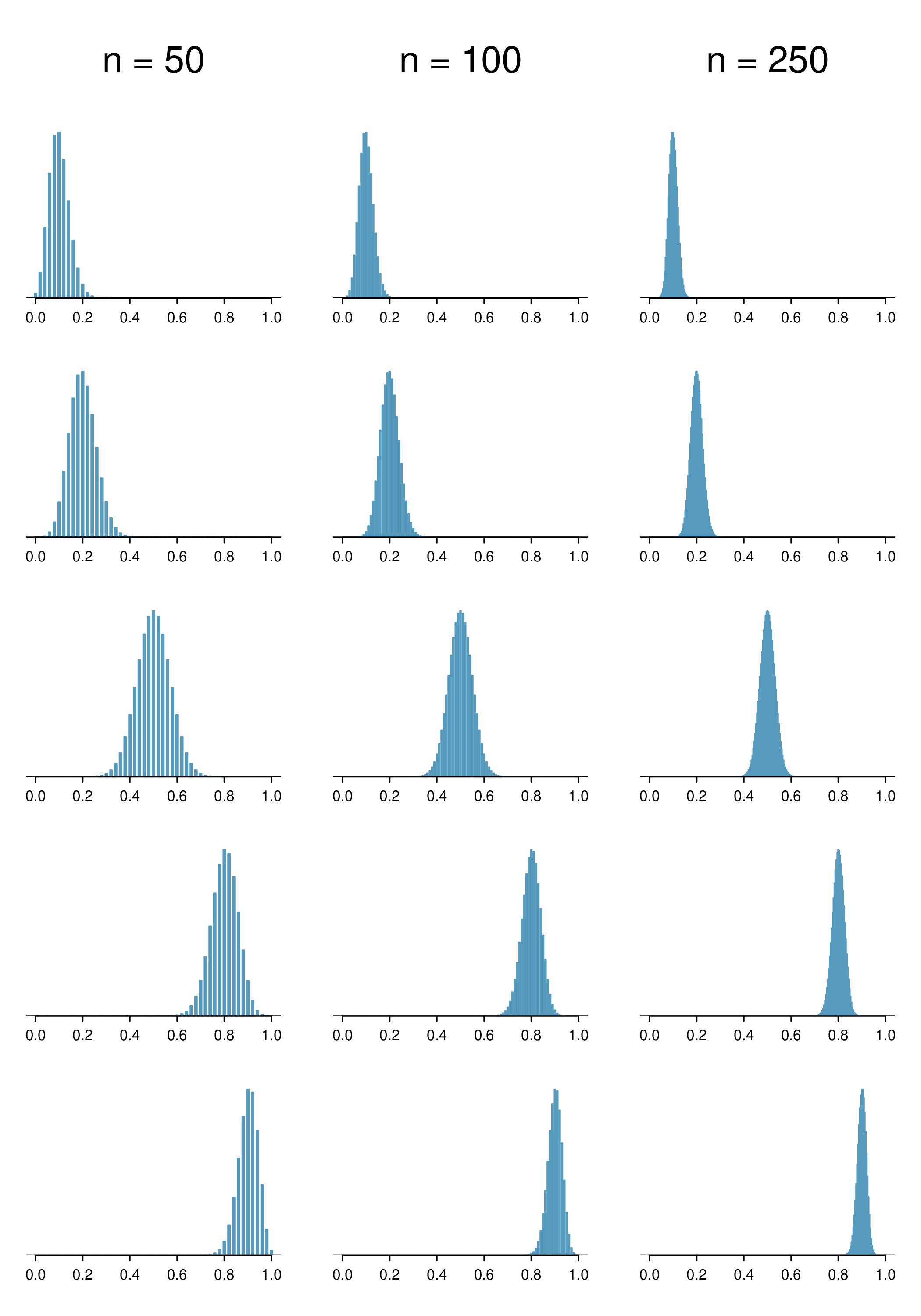
An interesting question to answer is, what happens when $np < 10$ or $n(1-p) < 10\text{?}$ As we did in Subsection 5.1.2, we can simulate drawing samples of different sizes where, say, the true proportion is $p = 0.25\text{.}$ Here’s a sample of size 10:

🔗

no, no, yes, yes, no, no, no, no, no, no
🔗

🔗

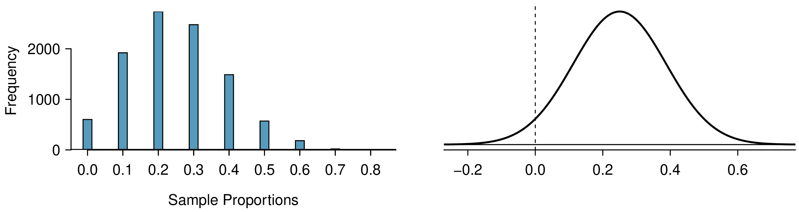
In this sample, we observe a sample proportion of yeses of $\hat{p} = \frac{2}{10} = 0.2\text{.}$ We can simulate many such proportions to understand the sampling distribution of $\hat{p}$ when $n = 10$ and $p = 0.25\text{,}$ which we’ve plotted in Figure 5.1.9 alongside a normal distribution with the same mean and variability. These distributions have a number of important differences.

🔗

There are two plots. The first plot is a histogram of 10,000 simulations of p-hat when the sample size is n equals 10 and the population proportion is p equals 0.25. The possible values are 0.0, 0.1, 0.2, and so on up to 1.0, though the graph only shows values up to 0.8. The distribution is centered at about 0.25, and is slightly right-skewed. The frequencies are about 500 for 0.0, 1900 for 0.1, 2800 for 0.2, 2400 for 0.3, 1500 for 0.4, 500 for 0.5, 100 for 0.6, and the bin heights for the remaining values have bin heights that are not visually distinguishable from zero. The second plot shows a normal distribution centered at 0.25 with a standard deviation of 0.137. The plot has a vertical line located at 0.0, which makes it more visually evident that a portion of the area under the normal distribution -- about 5% of this area -- represents values below 0.0. — Figure 5.1.9. Left: simulations of $\hat{p}$ when the sample size is $n = 10$ and the population proportion is $p = 0.25\text{.}$ Right: a normal distribution with the same mean (0.25) and standard deviation (0.137).
🔗

Figure 5.1.10 and Figure 5.1.11 show sampling distributions for several scenarios of $p$ and $n\text{.}$

🔗

Sampling distributions are shown for several scenarios for parameters p and n. The graphs are arranged in a grid of 5 rows representing proportions 0.1, 0.2, 0.5, 0.8, and 0.9 and 2 columns of sample sizes n equals 10 and 25. In each graph, the distribution is centered at the proportion. Given that these are proportions based on relatively small sample sizes, the bins do look relatively discrete (jumpy from one to the next), though less so for the distributions based on n equals 25. In cases where the true underlying proportion is near the lower bound of 0 or the upper bound of 1, the distribution tends to skew away from that boundary. This is most noticeable for both the distributions representing proportions closer to either boundary and for the smaller sample size. One distribution stands out among the 10 shown: the sample with p equals 0.5 and n equals 25, which shows a bell-shaped distribution resembling the normal distribution, though the data are still somewhat discrete. — Figure 5.1.10. Sampling distributions for several scenarios of $p$ and $n\text{.}$ Rows: $p = 0.10\text{,}$ $p = 0.20\text{,}$ $p = 0.50\text{,}$ $p = 0.80\text{,}$ and $p = 0.90\text{.}$ Columns: $n = 10$ and $n = 25\text{.}$
🔗

Table 5.1.12. Comparison of distributions

🔗

	Unimodal?	Smooth?	Symmetric?
Normal: $N(0.25, 0.14)$	Yes	Yes	Yes
$n = 10\text{,}$ $p = 0.25$	Yes	No	No

Notice that the success-failure condition was not satisfied when $n = 10$ and $p = 0.25\text{:}$

\begin{align*} np = 10 \times 0.25 = 2.5 \amp\amp n(1-p) = 10 \times 0.75 = 7.5 \end{align*}

This single sampling distribution does not show that the success-failure condition is the perfect guideline, but we have found that the guideline did correctly identify that a normal distribution might not be appropriate.

🔗

We can complete several additional simulations, shown in Figure 5.1.10 and Figure 5.1.11, and we can see some trends:

🔗

When either $np$ or $n(1-p)$ is small, the distribution is more discrete, i.e. not continuous.

🔗
When $np$ or $n(1-p)$ is smaller than 10, the skew in the distribution is more noteworthy.

🔗
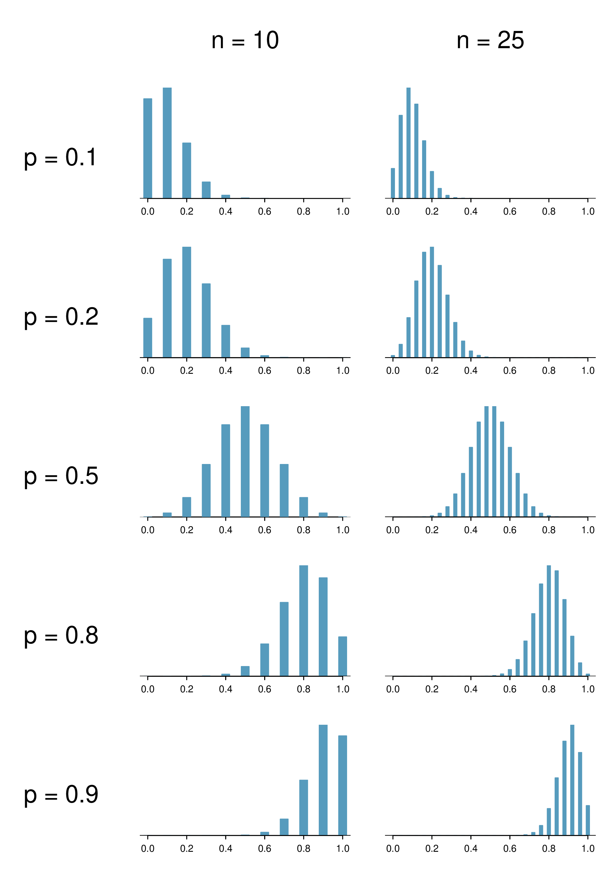
The larger both $np$ and $n(1-p)\text{,}$ the more normal the distribution. This may be a little harder to see for the larger sample size in these plots as the variability also becomes much smaller.

🔗
When $np$ and $n(1-p)$ are both very large, the distribution’s discreteness is hardly evident, and the distribution looks much more like a normal distribution.

🔗

So far we’ve only focused on the skew and discreteness of the distributions. We haven’t considered how the mean and standard error of the distributions change. Take a moment to look back at the graphs, and pay attention to three things:

🔗

The centers of the distribution are always at the population proportion, $p\text{,}$ that was used to generate the simulation. Because the sampling distribution of $\hat{p}$ is always centered at the population parameter $p\text{,}$ it means the sample proportion $\hat{p}$ is unbiased when the data are independent and drawn from such a population.

🔗
For a particular population proportion $p\text{,}$ the variability in the sampling distribution decreases as the sample size $n$ becomes larger. This will likely align with your intuition: an estimate based on a larger sample size will tend to be more accurate.

🔗
For a particular sample size, the variability will be largest when $p = 0.5\text{.}$ The differences may be a little subtle, so take a close look. This reflects the role of the proportion $p$ in the standard error formula: $SE = \sqrt{\frac{p(1-p)}{n}}\text{.}$ The standard error is largest when $p = 0.5\text{.}$

🔗

At no point will the distribution of $\hat{p}$ look perfectly normal, since $\hat{p}$ will always take discrete values ($x/n$). It is always a matter of degree, and we will use the standard success-failure condition with minimums of 10 for $np$ and $n(1-p)$ as our guideline within this book.

🔗

Subsection 5.1.6 Extending the framework for other statistics

The strategy of using a sample statistic to estimate a parameter is quite common, and it’s a strategy that we can apply to other statistics besides a proportion. For instance, if we want to estimate the average salary for graduates from a particular college, we could survey a random sample of recent graduates; in that example, we’d be using a sample mean $\bar{x}$ to estimate the population mean $\mu$ for all graduates. As another example, if we want to estimate the difference in product prices for two websites, we might take a random sample of products available on both sites, check the prices on each, and then compute the average difference; this strategy certainly would give us some idea of the actual difference through a point estimate.

🔗

While this chapter emphasizes a single proportion context, we’ll encounter many different contexts throughout this book where these methods will be applied. The principles and general ideas are the same, even if the details change a little. We’ve also sprinkled some other contexts into the exercises to help you start thinking about how the ideas generalize.

🔗

Exercises 5.1.7 Section 5.1 Exercises

1. Identify the parameter, Part I.

For each of the following situations, state whether the parameter of interest is a mean or a proportion. It may be helpful to examine whether individual responses are numerical or categorical.

🔗

In a survey, one hundred college students are asked how many hours per week they spend on the Internet.

🔗
In a survey, one hundred college students are asked: "What percentage of the time you spend on the Internet is part of your course work?"

🔗
In a survey, one hundred college students are asked whether or not they cited information from Wikipedia in their papers.

🔗
In a survey, one hundred college students are asked what percentage of their total weekly spending is on alcoholic beverages.

🔗
In a sample of one hundred recent college graduates, it is found that 85 percent expect to get a job within one year of their graduation date.

🔗

🔗

2. Identify the parameter, Part II.

For each of the following situations, state whether the parameter of interest is a mean or a proportion.

🔗

A poll shows that 64% of Americans personally worry a great deal about federal spending and the budget deficit.

🔗
A survey reports that local TV news has shown a 17% increase in revenue within a two year period while newspaper revenues decreased by 6.4% during this time period.

🔗
In a survey, high school and college students are asked whether or not they use geolocation services on their smart phones.

🔗
In a survey, smart phone users are asked whether or not they use a web-based taxi service.

🔗
In a survey, smart phone users are asked how many times they used a web-based taxi service over the last year.

🔗

🔗

3. Quality control.

As part of a quality control process for computer chips, an engineer at a factory randomly samples 212 chips during a week of production to test the current rate of chips with severe defects. She finds that 27 of the chips are defective.

🔗

What population is under consideration in the data set?

🔗
What parameter is being estimated?

🔗
What is the point estimate for the parameter?

🔗
What is the name of the statistic we use to measure the uncertainty of the point estimate?

🔗
Compute this value for this context.

🔗
The historical rate of defects is 10%. Should the engineer be surprised by the observed rate of defects during the current week?

🔗
Suppose the true population value was found to be 10%. If we use this proportion to recompute the value in part (e) using $p = 0.1$ instead of $\hat{p}\text{,}$ does the resulting value change much?

🔗

🔗

4. Unexpected expense.

In a random sample of 765 adults in the United States, 322 say they could not cover a $400 unexpected expense without borrowing money or going into debt.

🔗

What population is under consideration in the data set?

🔗
What parameter is being estimated?

🔗
What is the point estimate for the parameter?

🔗
What is the name of the statistic we use to measure the uncertainty of the point estimate?

🔗
Compute the value from part (d) for this context.

🔗
A cable news pundit thinks the value is actually 50%. Should she be surprised by the data?

🔗
Suppose the true population value was found to be 40%. If we use this proportion to recompute the value in part (e) using $p = 0.4$ instead of $\hat{p}\text{,}$ does the resulting value change much?

🔗

🔗

5. Repeated water samples.

A nonprofit wants to understand the fraction of households that have elevated levels of lead in their drinking water. They expect at least 5% of homes will have elevated levels of lead, but not more than about 30%. They randomly sample 800 homes and work with the owners to retrieve water samples, and they compute the fraction of these homes with elevated lead levels. They repeat this 1,000 times and build a distribution of sample proportions.

🔗

What is this distribution called?

🔗
Would you expect the shape of this distribution to be symmetric, right skewed, or left skewed? Explain your reasoning.

🔗
If the proportions are distributed around 8%, what is the variability of the distribution?

🔗
What is the formal name of the value you computed in (c)?

🔗
Suppose the researchers’ budget is reduced, and they are only able to collect 250 observations per sample, but they can still collect 1,000 samples. They build a new distribution of sample proportions. How will the variability of this new distribution compare to the variability of the distribution when each sample contained 800 observations?

🔗

🔗

6. Repeated student samples.

Of all freshman at a large college, 16% made the dean’s list in the current year. As part of a class project, students randomly sample 40 students and check if those students made the list. They repeat this 1,000 times and build a distribution of sample proportions.

🔗

What is this distribution called?

🔗
Would you expect the shape of this distribution to be symmetric, right skewed, or left skewed? Explain your reasoning.

🔗
Calculate the variability of this distribution.

🔗
What is the formal name of the value you computed in (c)?

🔗
Suppose the students decide to sample again, this time collecting 90 students per sample, and they again collect 1,000 samples. They build a new distribution of sample proportions. How will the variability of this new distribution compare to the variability of the distribution when each sample contained 40 observations?

🔗

🔗

Prev Top Next

	Unimodal?	Smooth?	Symmetric?
Normal: \(N(0.25, 0.14)\)	Yes	Yes	Yes
\(n = 10\text{,}\) \(p = 0.25\)	Yes	No	No