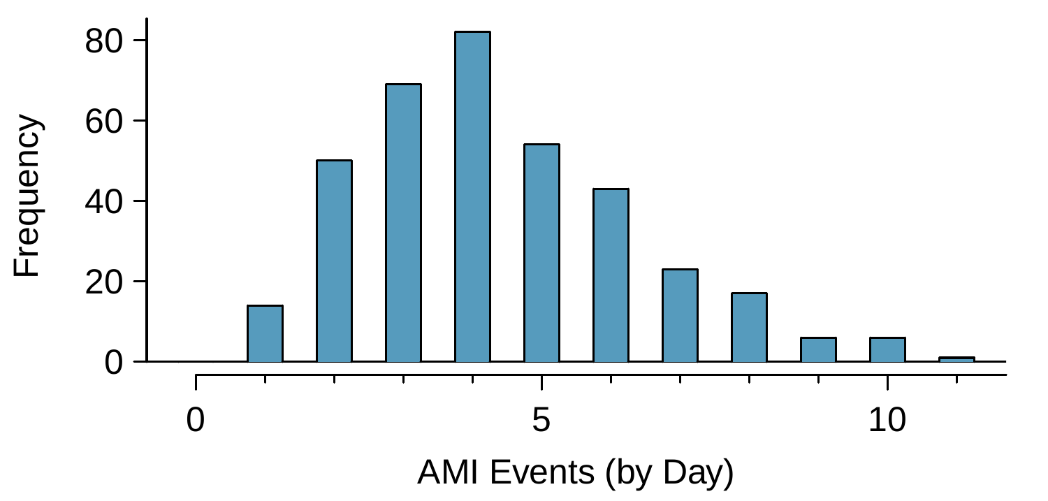
There are about 8 million individuals in New York City. How many individuals might we expect to be hospitalized for acute myocardial infarction (AMI), i.e. a heart attack, each day? According to historical records, the average number is about 4.4 individuals. However, we would also like to know the approximate distribution of counts. What would a histogram of the number of AMI occurrences each day look like if we recorded the daily counts over an entire year?
A histogram of the number of occurrences of AMI on 365 days for NYC is shown in Figure 4.5.2. 1
These data are simulated. In practice, we should check for an association between successive days.
The sample mean (4.38) is similar to the historical average of 4.4. The sample standard deviation is about 2, and the histogram indicates that about 70% of the data fall between 2.4 and 6.4. The distribution’s shape is unimodal and skewed to the right.
The Poisson distribution is often useful for estimating the number of events in a large population over a unit of time. For instance, consider each of the following events:
The Poisson distribution helps us describe the number of such events that will occur in a day for a fixed population if the individuals within the population are independent. The Poisson distribution could also be used over another unit of time, such as an hour or a week.
The histogram in Figure 4.5.2 approximates a Poisson distribution with rate equal to 4.4. The rate for a Poisson distribution is the average number of occurrences in a mostly-fixed population per unit of time. In Example 4.5.1, the time unit is a day, the population is all New York City residents, and the historical rate is 4.4. The parameter in the Poisson distribution is the rate—or how many events we expect to observe—and it is typically denoted by \(\lambda\) (the Greek letter lambda) or \(\mu\text{.}\) Using the rate, we can describe the probability of observing exactly \(k\) events in a single unit of time.
where \(k\) may take a value 0, 1, 2, and so on, and \(k!\) represents \(k\)-factorial, as described on page Section 4.3. The letter \(e \approx 2.718\) is the base of the natural logarithm. The mean and standard deviation of this distribution are \(\lambda\) and \(\sqrt{\lambda}\text{,}\) respectively.
We will leave a rigorous set of conditions for the Poisson distribution to a later course. However, we offer a few simple guidelines that can be used for an initial evaluation of whether the Poisson model would be appropriate.
A random variable may follow a Poisson distribution if we are looking for the number of events, the population that generates such events is large, and the events occur independently of each other.
Even when events are not really independent—for instance, Saturdays and Sundays are especially popular for weddings—a Poisson model may sometimes still be reasonable if we allow it to have a different rate for different times. In the wedding example, the rate would be modeled as higher on weekends than on weekdays. The idea of modeling rates for a Poisson distribution against a second variable such as the day of week forms the foundation of some more advanced methods that fall in the realm of generalized linear models. In Chapter 8 and Chapter 9, we will discuss a foundation of linear models.
Which distribution have we studied that is most appropriate for calculating the probability of a given number of customers arriving within one hour during this time of day?
For Monday through Thursday when there isn’t a holiday, the average number of vehicles that visit a particular retailer between 2pm and 3pm each afternoon is 6.5, and the number of cars that show up on any given day follows a Poisson distribution.
There is an average of 11.7 people who visit during those same hours from vehicles. Is it likely that the number of people visiting by car during this hour is also Poisson? Explain.
Occasionally an airline will lose a bag. Suppose a small airline has found it can reasonably model the number of bags lost each weekday using a Poisson model with a mean of 2.2 bags.
Suppose the airline expands over the course of the next 3 years, doubling the number of flights it makes, and the CEO asks you if it’s reasonable for them to continue using the Poisson model with a mean of 2.2. What is an appropriate recommendation? Explain.