A group of researchers are interested in the possible effects of distracting stimuli during eating, such as an increase or decrease in the amount of food consumption. To test this hypothesis, they monitored food intake for a group of 44 patients who were randomized into two equal groups. The treatment group ate lunch while playing solitaire, and the control group ate lunch without any added distractions. Patients in the treatment group ate 52.1 grams of biscuits, with a standard deviation of 45.1 grams, and patients in the control group ate 27.1 grams of biscuits, with a standard deviation of 26.4 grams. Do these data provide convincing evidence that the average food intake (measured in amount of biscuits consumed) is different for the patients in the treatment group? Assume that conditions for inference are satisfied.
The researchers from Exercise 7.6.1 also investigated the effects of being distracted by a game on how much people eat. The 22 patients in the treatment group who ate their lunch while playing solitaire were asked to do a serial-order recall of the food lunch items they ate. The average number of items recalled by the patients in this group was 4.9, with a standard deviation of 1.8. The average number of items recalled by the patients in the control group (no distraction) was 6.1, with a standard deviation of 1.8. Do these data provide strong evidence that the average number of food items recalled by the patients in the treatment and control groups are different?
Determine if the following statement is true or false, and if false, explain your reasoning: If comparing means of two groups with equal sample sizes, always use a paired test.
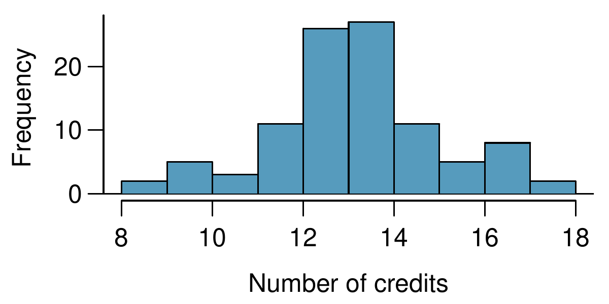
A college counselor is interested in estimating how many credits a student typically enrolls in each semester. The counselor decides to randomly sample 100 students by using the registrar’s database of students. The histogram below shows the distribution of the number of credits taken by these students. Sample statistics for this distribution are also provided.
The college counselor takes another random sample of 100 students and this time finds a sample mean of 14.02 credits. Should she be surprised that this sample statistic is slightly different than the one from the original sample? Explain your reasoning.
The sample means given above are point estimates for the mean number of credits taken by all students at that college. What measures do we use to quantify the variability of this estimate? Compute this quantity using the data from the original sample.
The distribution of the number of eggs laid by a certain species of hen during their breeding period has a mean of 35 eggs with a standard deviation of 18.2. Suppose a group of researchers randomly samples 45 hens of this species, counts the number of eggs laid during their breeding period, and records the sample mean. They repeat this 1,000 times, and build a distribution of sample means.
Suppose the researchers’ budget is reduced and they are only able to collect random samples of 10 hens. The sample mean of the number of eggs is recorded, and we repeat this 1,000 times, and build a new distribution of sample means. How will the variability of this new distribution compare to the variability of the original distribution?
Forest rangers wanted to better understand the rate of growth for younger trees in the park. They took measurements of a random sample of 50 young trees in 2009 and again measured those same trees in 2019. The data below summarize their measurements, where the heights are in feet:
At a startup company running a new weather app, an engineering team generally runs experiments where a random sample of 1% of the app’s visitors in the control group and another 1% were in the treatment group to test each new feature. The team’s core goal is to increase a metric called daily visitors, which is essentially the number of visitors to the app each day. They track this metric in each experiment arm and as their core experiment metric. In their most recent experiment, the team tested including a new animation when the app started, and the number of daily visitors in this experiment stabilized at +1.2% with a 95% confidence interval of (-0.2%, +2.6%). This means if this new app start animation was launched, the team thinks they might lose as many as 0.2% of daily visitors or gain as many as 2.6% more daily visitors. Suppose you are consulting as the team’s data scientist, and after discussing with the team, you and they agree that they should run another experiment that is bigger. You also agree that this new experiment should be able to detect a gain in the daily visitors metric of 1.0% or more with 80% power. Now they turn to you and ask, “How big of an experiment do we need to run to ensure we can detect this effect?”
How small must the standard error be if the team is to be able to detect an effect of 1.0% with 80% power and a significance level of \(\alpha = 0.05\text{?}\) You may safely assume the percent change in daily visitors metric follows a normal distribution.
Consider the first experiment, where the point estimate was +1.2% and the 95% confidence interval was (-0.2%, +2.6%). If that point estimate followed a normal distribution, what was the standard error of the estimate?
The ratio of the standard error from part (a) vs the standard error from part (b) should be 1.97. How much bigger of an experiment is needed to shrink a standard error by a factor of 1.97?
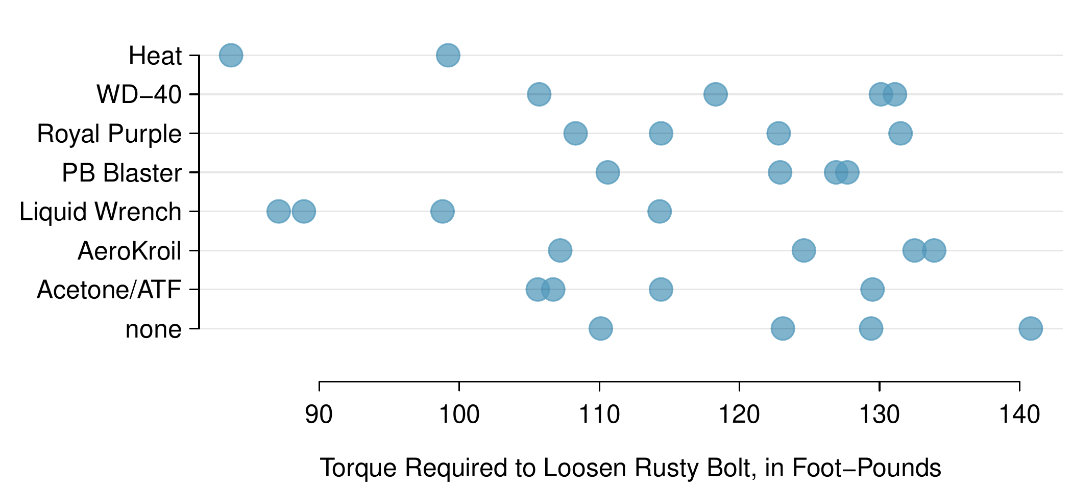
Project Farm is a YouTube channel that routinely compares different products. In one episode, the channel evaluated different options for loosening rusty bolts. Eight options were evaluated, including a control group where no treatment was given (“none” in the graph), to determine which was most effective. For all treatments, there were four bolts tested, except for a treatment of heat with a blow torch, where only two data points were collected. The results are shown in the figure below:
Regardless of your answer in part (a), describe hypotheses for ANOVA in this context, and use the table below to carry out the test. Give your conclusion in the context of the data.
The table below are p-values for pairwise \(t\)-tests comparing each of the different groups. These p-values have not been corrected for multiple comparisons. Which pair of groups appears most likely to represent a difference?
There are 28 p-values shown in the table in part (c). Determine if any of them are statistically significant after correcting for multiple comparisons. If so, which one(s)? Explain your answer.
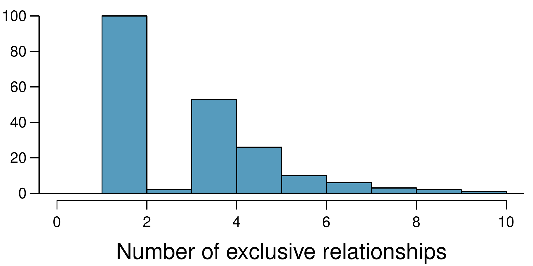
A survey conducted on a reasonably random sample of 203 undergraduates asked, among many other questions, about the number of exclusive relationships these students have been in. The histogram below shows the distribution of the data from this sample. The sample average is 3.2 with a standard deviation of 1.97.
Estimate the average number of exclusive relationships students have been in using a 90% confidence interval and interpret this interval in context. Check any conditions required for inference, and note any assumptions you must make as you proceed with your calculations and conclusions.
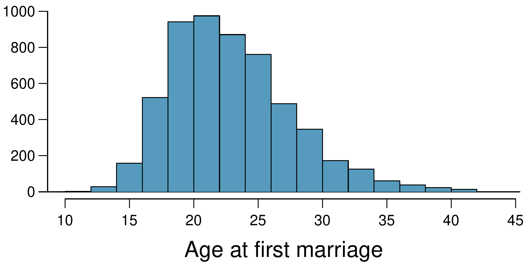
The National Survey of Family Growth conducted by the Centers for Disease Control gathers information on family life, marriage and divorce, pregnancy, infertility, use of contraception, and men’s and women’s health. One of the variables collected on this survey is the age at first marriage. The histogram below shows the distribution of ages at first marriage of 5,534 randomly sampled women between 2006 and 2010. The average age at first marriage among these women is 23.44 with a standard deviation of 4.72.
Estimate the average age at first marriage of women using a 95% confidence interval, and interpret this interval in context. Discuss any relevant assumptions.
A study suggests that the average college student spends 10 hours per week communicating with others online. You believe that this is an underestimate and decide to collect your own sample for a hypothesis test. You randomly sample 60 students from your dorm and find that on average they spent 13.5 hours a week communicating with others online. A friend of yours, who offers to help you with the hypothesis test, comes up with the following set of hypotheses. Indicate any errors you see.
Exercise 7.6.10 presents the results of a 2006 - 2010 survey showing that the average age of women at first marriage is 23.44. Suppose a social scientist thinks this value has changed since the survey was taken. Below is how she set up her hypotheses. Indicate any errors you see.