Introductory Statistics

Section 5.3 Hypothesis Testing for a Proportion

The following question comes from a book written by Hans Rosling, Anna Rosling RΓΆnnlund, and Ola Rosling called Factfulness:
How many of the world’s 1 year old children today have been vaccinated against some disease:
  1. 20%
  2. 50%
  3. 80%
Write down what your answer (or guess), and when you’re ready, find the answer in the footnote.
 1 
The correct answer is (c): 80% of the world’s 1 year olds have been vaccinated against some disease.
In this section, we’ll be exploring how people with a 4-year college degree perform on this and other world health questions as we learn about hypothesis tests, which are a framework used to rigorously evaluate competing ideas and claims.

Subsection 5.3.1 Hypothesis testing framework

We’re interested in understanding how much people know about world health and development. If we take a multiple choice world health question, then we might like to understand if
\(\mathbf{H_0}\text{:}\)
People never learn these particular topics and their responses are simply equivalent to random guesses.
\(\mathbf{H_A}\text{:}\)
People have knowledge that helps them do better than random guessing, or perhaps, they have false knowledge that leads them to actually do worse than random guessing.
These competing ideas are called hypotheses. We call \(H_0\) the null hypothesis and \(H_A\) the alternative hypothesis. When there is a subscript 0 like in \(H_0\text{,}\) data scientists pronounce it as β€œnought” (e.g. \(H_0\) is pronounced β€œH-nought”).

Null and alternative hypotheses.

The null hypothesis (\(H_0\)) often represents a skeptical perspective or a claim to be tested. The alternative hypothesis (\(H_A\)) represents an alternative claim under consideration and is often represented by a range of possible parameter values.
Our job as data scientists is to play the role of a skeptic: before we buy into the alternative hypothesis, we need to see strong supporting evidence.
The null hypothesis often represents a skeptical position or a perspective of β€œno difference”. In our first example, we’ll consider whether the typical person does any different than random guessing on Roslings’ question about infant vaccinations.
The alternative hypothesis generally represents a new or stronger perspective. In the case of the question about infant vaccinations, it would certainly be interesting to learn whether people do better than random guessing, since that would mean that the typical person knows something about world health statistics. It would also be very interesting if we learned that people do worse than random guessing, which would suggest people believe incorrect information about world health.
The hypothesis testing framework is a very general tool, and we often use it without a second thought. If a person makes a somewhat unbelievable claim, we are initially skeptical. However, if there is sufficient evidence that supports the claim, we set aside our skepticism and reject the null hypothesis in favor of the alternative. The hallmarks of hypothesis testing are also found in the US court system.

Checkpoint 5.3.1.

A US court considers two possible claims about a defendant: she is either innocent or guilty. If we set these claims up in a hypothesis framework, which would be the null hypothesis and which the alternative?
Solution.
The jury considers whether the evidence is so convincing (strong) that there is no reasonable doubt regarding the person’s guilt; in such a case, the jury rejects innocence (the null hypothesis) and concludes the defendant is guilty (alternative hypothesis).
Jurors examine the evidence to see whether it convincingly shows a defendant is guilty. Even if the jurors leave unconvinced of guilt beyond a reasonable doubt, this does not mean they believe the defendant is innocent. This is also the case with hypothesis testing: even if we fail to reject the null hypothesis, we typically do not accept the null hypothesis as true. Failing to find strong evidence for the alternative hypothesis is not equivalent to accepting the null hypothesis.
When considering Roslings’ question about infant vaccination, the null hypothesis represents the notion that the people we will be considering -- college-educated adults -- are as accurate as random guessing. That is, the proportion \(p\) of respondents who pick the correct answer, that 80% of 1 year olds have been vaccinated against some disease, is about 33.3% (or 1-in-3 if wanting to be perfectly precise). The alternative hypothesis is that this proportion is something other than 33.3%. While it’s helpful to write these hypotheses in words, it can be useful to write them using mathematical notation:
\(H_0\text{:}\)
\(\displaystyle p = 0.333\)
\(H_A\text{:}\)
\(\displaystyle p \neq 0.333\)
In this hypothesis setup, we want to make a conclusion about the population parameter \(p\text{.}\) The value we are comparing the parameter to is called the null value, which in this case is 0.333. It’s common to label the null value with the same symbol as the parameter but with a subscript `0’. That is, in this case, the null value is \(p_0 = 0.333\) (pronounced β€œp-nought equals 0.333”).

Example 5.3.2.

It may seem impossible that the proportion of people who get the correct answer is exactly 33.3%. If we don’t believe the null hypothesis, should we simply reject it?
Solution.
No. While we may not buy into the notion that the proportion is exactly 33.3%, the hypothesis testing framework requires that there be strong evidence before we reject the null hypothesis and conclude something more interesting.
After all, even if we don’t believe the proportion is exactly 33.3%, that doesn’t really tell us anything useful! We would still be stuck with the original question: do people do better or worse than random guessing on Roslings’ question? Without data that strongly points in one direction or the other, it is both uninteresting and pointless to reject \(H_0\text{.}\)

Checkpoint 5.3.3.

Another example of a real-world hypothesis testing situation is evaluating whether a new drug is better or worse than an existing drug at treating a particular disease. What should we use for the null and alternative hypotheses in this case?
Solution.
The null hypothesis (\(H_0\)) in this case is the declaration of no difference: the drugs are equally effective. The alternative hypothesis (\(H_A\)) is that the new drug performs differently than the original, i.e. it could perform better or worse.

Subsection 5.3.2 Testing hypotheses using confidence intervals

We will use the Rosling responses data set to evaluate the hypothesis test evaluating whether college-educated adults who get the question about infant vaccination correct is different from 33.3%. This data set summarizes the answers of 50 college-educated adults. Of these 50 adults, 24% of respondents got the question correct that 80% of 1 year olds have been vaccinated against some disease.
Up until now, our discussion has been philosophical. However, now that we have data, we might ask ourselves: does the data provide strong evidence that the proportion of all college-educated adults who would answer this question correctly is different than 33.3%?
We learned in SectionΒ 5.1 that there is fluctuation from one sample to another, and it is unlikely that our sample proportion, \(\hat{p}\text{,}\) will exactly equal \(p\text{,}\) but we want to make a conclusion about \(p\text{.}\) We have a nagging concern: is this deviation of 24% from 33.3% simply due to chance, or does the data provide strong evidence that the population proportion is different from 33.3%?
In SectionΒ 5.2, we learned how to quantify the uncertainty in our estimate using confidence intervals. The same method for measuring variability can be useful for the hypothesis test.

Example 5.3.4.

Check whether it is reasonable to construct a confidence interval for \(p\) using the sample data, and if so, construct a 95% confidence interval.
Solution.
The conditions are met for \(\hat{p}\) to be approximately normal: the data come from a simple random sample (satisfies independence), and \(n\hat{p} = 12\) and \(n(1 - \hat{p}) = 38\) are both at least 10 (success-failure condition).
To construct the confidence interval, we will need to identify the point estimate (\(\hat{p} = 0.24\)), the critical value for the 95% confidence level (\(z^{\star} = 1.96\)), and the standard error of \(\hat{p}\) (\(SE_{\hat{p}} = \sqrt{\hat{p}(1 - \hat{p}) / n} = 0.060\)). With those pieces, the confidence interval for \(p\) can be constructed:
\begin{align*} \amp\hat{p} \pm z^{\star} \times SE_{\hat{p}}\\ \amp 0.24 \pm 1.96 \times 0.060\\ \amp (0.122, 0.358) \end{align*}
We are 95% confident that the proportion of all college-educated adults to correctly answer this particular question about infant vaccination is between 12.2% and 35.8%.
Because the null value in the hypothesis test is \(p_0 = 0.333\text{,}\) which falls within the range of plausible values from the confidence interval, we cannot say the null value is implausible.
 2 
Arguably this method is slightly imprecise. As we’ll see in a few pages, the standard error is often computed slightly differently in the context of a hypothesis test for a proportion.
That is, the data do not provide sufficient evidence to reject the notion that the performance of college-educated adults was different than random guessing, and we do not reject the null hypothesis, \(H_0\text{.}\)

Example 5.3.5.

Explain why we cannot conclude that college-educated adults simply guessed on the infant vaccination question.
Solution.
While we failed to reject \(H_0\text{,}\) that does not necessarily mean the null hypothesis is true. Perhaps there was an actual difference, but we were not able to detect it with the relatively small sample of 50.

Double negatives can sometimes be used in statistics.

In many statistical explanations, we use double negatives. For instance, we might say that the null hypothesis is not implausible or we failed to reject the null hypothesis. Double negatives are used to communicate that while we are not rejecting a position, we are also not saying it is correct.

Checkpoint 5.3.6.

Let’s move onto a second question posed by the Roslings:
There are 2 billion children in the world today aged 0-15 years old, how many children will there be in year 2100 according to the United Nations?
  1. 4 billion.
  2. 3 billion.
  3. 2 billion.
Set up appropriate hypotheses to evaluate whether college-educated adults are better than random guessing on this question. Also, see if you can guess the correct answer before checking the answer in the solution!
Solution.
The appropriate hypotheses are:
\(H_0\text{:}\) the proportion who get the answer correct is the same as random guessing: 1-in-3, or \(p = 0.333\text{.}\)
\(H_A\text{:}\) the proportion who get the answer correct is different than random guessing, \(p \neq 0.333\text{.}\)
The correct answer to the question is 2 billion. While the world population is projected to increase, the average age is also expected to rise. That is, the majority of the population growth will happen in older age groups, meaning people are projected to live longer in the future across much of the world.

Checkpoint 5.3.7.

This time we took a larger sample of 228 college-educated adults, 34 (14.9%) selected the correct answer to the question above: 2 billion. Can we model the sample proportion using a normal distribution and construct a confidence interval?
Solution.
We check both conditions, which are satisfied, so it is reasonable to use a normal distribution for \(\hat{p}\text{:}\)
Independence. Since the data are from a simple random sample, the observations are independent.
Success-failure. We’ll use \(\hat{p}\) in place of \(p\) to check: \(n\hat{p} = 34\) and \(n(1 - \hat{p}) = 194\text{.}\) Both are greater than 10, so the success-failure condition is satisfied.

Example 5.3.8.

Compute a 95% confidence interval for the fraction of college-educated adults who answered the children-in-2100 question correctly, and evaluate the hypotheses from the previous exercise.
Solution.
To compute the standard error, we’ll again use \(\hat{p}\) in place of \(p\) for the calculation:
\begin{align*} SE_{\hat{p}} \amp= \sqrt{\frac{\hat{p}(1 - \hat{p})}{n}}\\ \amp= \sqrt{\frac{0.149(1 - 0.149)} {228}}\\ \amp= 0.024 \end{align*}
In the previous exercise, we found that \(\hat{p}\) can be modeled using a normal distribution, which ensures a 95% confidence interval may be accurately constructed as
\begin{align*} \hat{p}\ \amp\pm\ z^{\star} \times SE\\ \amp\quad\to\quad 0.149\ \pm\ 1.96 \times 0.024\\ \amp\quad\to\quad (0.103, 0.195) \end{align*}
Because the null value, \(p_0 = 0.333\text{,}\) is not in the confidence interval, a population proportion of 0.333 is implausible and we reject the null hypothesis. That is, the data provide statistically significant evidence that the actual proportion of college adults who get the children-in-2100 question correct is different from random guessing. Because the entire 95% confidence interval is below 0.333, we can conclude college-educated adults do worse than random guessing on this question.
One subtle consideration is that we used a 95% confidence interval. What if we had used a 99% confidence level? Or even a 99.9% confidence level? It’s possible to come to a different conclusion if using a different confidence level. Therefore, when we make a conclusion based on confidence interval, we should also be sure it is clear what confidence level we used.
The worse-than-random performance on this last question is not a fluke: there are many such world health questions where people do worse than random guessing. In general, the answers suggest that people tend to be more pessimistic about progress than reality suggests. This topic is discussed in much greater detail in the Roslings’ book, Factfulness.

Subsection 5.3.3 Decision errors

Hypothesis tests are not flawless: we can make an incorrect decision in a statistical hypothesis test based on the data. For example, in the court system innocent people are sometimes wrongly convicted and the guilty sometimes walk free. One key distinction with statistical hypothesis tests is that we have the tools necessary to probabilistically quantify how often we make errors in our conclusions.
Recall that there are two competing hypotheses: the null and the alternative. In a hypothesis test, we make a statement about which one might be true, but we might choose incorrectly. There are four possible scenarios, which are summarized in TableΒ 5.3.9.
Table 5.3.9. Four different scenarios for hypothesis tests.
Test conclusion
do not reject \(H_0\) reject \(H_0\) in favor of \(H_A\)
\(H_0\) true okay Type 1 Error
Truth \(H_A\) true Type 2 Error okay
A Type 1 Error is rejecting the null hypothesis when \(H_0\) is actually true. A Type 2 Error is failing to reject the null hypothesis when the alternative is actually true.

Checkpoint 5.3.10.

In a US court, the defendant is either innocent (\(H_0\)) or guilty (\(H_A\)). What does a Type 1 Error represent in this context? What does a Type 2 Error represent? TableΒ 5.3.9 may be useful.
Solution.
If the court makes a Type 1 Error, this means the defendant is innocent (\(H_0\) true) but wrongly convicted. Note that a Type 1 Error is only possible if we’ve rejected the null hypothesis.
A Type 2 Error means the court failed to reject \(H_0\) (i.e. failed to convict the person) when she was in fact guilty (\(H_A\) true). Note that a Type 2 Error is only possible if we have failed to reject the null hypothesis.

Example 5.3.11.

How could we reduce the Type 1 Error rate in US courts? What influence would this have on the Type 2 Error rate?
Solution.
To lower the Type 1 Error rate, we might raise our standard for conviction from β€œbeyond a reasonable doubt” to β€œbeyond a conceivable doubt” so fewer people would be wrongly convicted. However, this would also make it more difficult to convict the people who are actually guilty, so we would make more Type 2 Errors.

Checkpoint 5.3.12.

How could we reduce the Type 2 Error rate in US courts? What influence would this have on the Type 1 Error rate?
Solution.
To lower the Type 2 Error rate, we want to convict more guilty people. We could lower the standards for conviction from β€œbeyond a reasonable doubt” to β€œbeyond a little doubt”. Lowering the bar for guilt will also result in more wrongful convictions, raising the Type 1 Error rate.
The previous exercises provide an important lesson: if we reduce how often we make one type of error, we generally make more of the other type.
Hypothesis testing is built around rejecting or failing to reject the null hypothesis. That is, we do not reject \(H_0\) unless we have strong evidence. But what precisely does strong evidence mean? As a general rule of thumb, for those cases where the null hypothesis is actually true, we do not want to incorrectly reject \(H_0\) more than 5% of the time. This corresponds to a significance level of 0.05. That is, if the null hypothesis is true, the significance level indicates how often the data lead us to incorrectly reject \(H_0\text{.}\) We often write the significance level using \(\alpha\) (the Greek letter alpha): \(\alpha = 0.05\text{.}\) We discuss the appropriateness of different significance levels in SubsectionΒ 5.3.5.
If we use a 95% confidence interval to evaluate a hypothesis test and the null hypothesis happens to be true, we will make an error whenever the point estimate is at least 1.96 standard errors away from the population parameter. This happens about 5% of the time (2.5% in each tail). Similarly, using a 99% confidence interval to evaluate a hypothesis is equivalent to a significance level of \(\alpha = 0.01\text{.}\)
A confidence interval is very helpful in determining whether or not to reject the null hypothesis. However, the confidence interval approach isn’t always sustainable. In several sections, we will encounter situations where a confidence interval cannot be constructed. For example, if we wanted to evaluate the hypothesis that several proportions are equal, it isn’t clear how to construct and compare many confidence intervals altogether.
Next we will introduce a statistic called the p-value to help us expand our statistical toolkit, which will enable us to both better understand the strength of evidence and work in more complex data scenarios in later sections.

Subsection 5.3.4 Formal Testing Using P-values

The p-value is a way of quantifying the strength of the evidence against the null hypothesis and in favor of the alternative hypothesis. Statistical hypothesis testing typically uses the p-value method rather than making a decision based on confidence intervals.

Definition 5.3.13. P-value.

The p-value is the probability of observing data at least as favorable to the alternative hypothesis as our current data set, if the null hypothesis were true. We typically use a summary statistic of the data, in this section the sample proportion, to help compute the p-value and evaluate the hypotheses.

Example 5.3.14. Setting up hypotheses for coal energy support.

Pew Research asked a random sample of 1000 American adults whether they supported the increased usage of coal to produce energy. Set up hypotheses to evaluate whether a majority of American adults support or oppose the increased usage of coal.
Solution.
The uninteresting result is that there is no majority either way: half of Americans support and the other half oppose expanding the use of coal to produce energy. The alternative hypothesis would be that there is a majority support or oppose (though we do not known which one!) expanding the use of coal. If \(p\) represents the proportion supporting, then we can write the hypotheses as
\begin{align*} H_0: \amp\ p = 0.5\\ H_A: \amp\ p \neq 0.5 \end{align*}
In this case, the null value is \(p_0 = 0.5\text{.}\)
When evaluating hypotheses for proportions using the p-value method, we will slightly modify how we check the success-failure condition and compute the standard error for the single proportion case. These changes aren’t dramatic, but pay close attention to how we use the null value, \(p_0\text{.}\)

Example 5.3.15. Constructing the null distribution for coal energy support.

Pew Research’s sample show that 37% of American adults support increased usage of coal. We now wonder, does 37% represent a real difference from the null hypothesis of 50%? What would the sampling distribution of \(\hat{p}\) look like if the null hypothesis were true?
Solution.
If the null hypothesis were true, the population proportion would be the null value, 0.5. We previously learned that the sampling distribution of \(\hat{p}\) will be normal when two conditions are met:
Independence.
The poll was based on a simple random sample, so independence is satisfied.
Success-failure.
Based on the poll’s sample size of \(n = 1000\text{,}\) the success-failure condition is met, since
\begin{gather*} np ~ \stackrel{H_0}{=} ~ 1000 \times 0.5 = 500 \qquad\qquad n(1-p) ~ \stackrel{H_0}{=} ~ 1000 \times (1-0.5) = 500 \end{gather*}
are both at least 10. Note that the success-failure condition was checked using the null value, \(p_0 = 0.5\text{;}\) this is the first procedural difference from confidence intervals.
If the null hypothesis were true, the sampling distribution indicates that a sample proportion based on \(n = 1000\) observations would be normally distributed. Next, we can compute the standard error, where we will again use the null value \(p_0 = 0.5\) in the calculation:
\begin{equation*} SE_{\hat{p}} = \sqrt{\frac{p(1-p)}{n}} \quad \stackrel{H_0}{=} \quad \sqrt{\frac{0.5 \times (1-0.5)}{1000}} = 0.016 \end{equation*}
This marks the other procedural difference from confidence intervals: since the sampling distribution is determined under the null proportion, the null value \(p_0\) was used for the proportion in the calculation rather than \(\hat{p}\text{.}\)
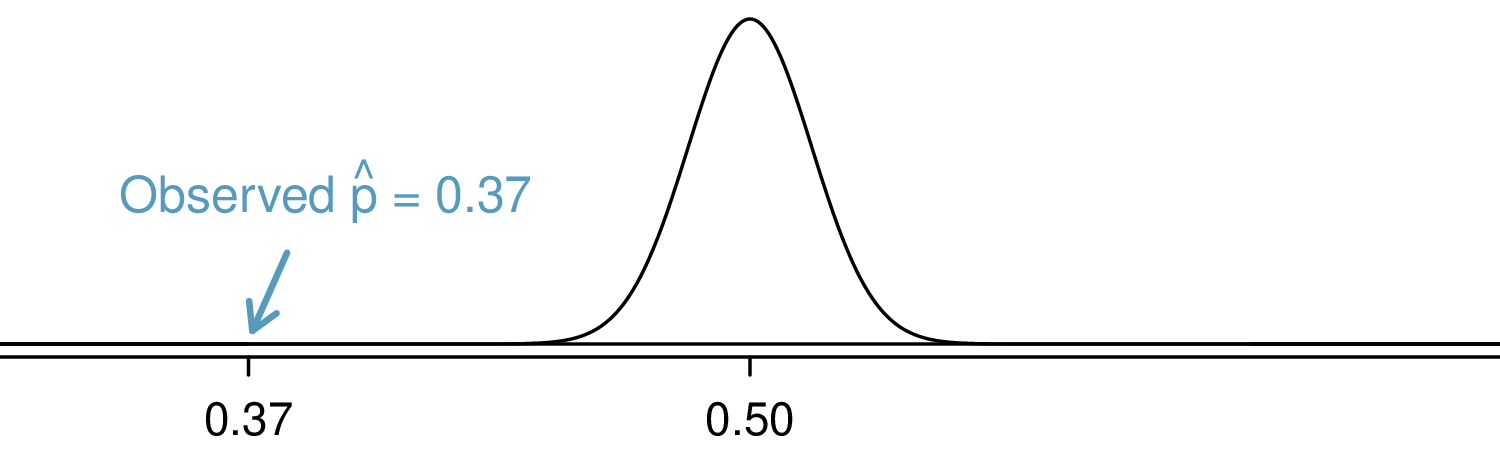
Ultimately, if the null hypothesis were true, then the sample proportion should follow a normal distribution with mean 0.5 and a standard error of 0.016. This distribution is shown in FigureΒ 5.3.16.
A normal distribution centered at 0.5 with a standard deviation of 0.016 is shown. Additionally, an annotation is located at 0.37 that states, "Observed p-hat equals 0.37".
Figure 5.3.16. If the null hypothesis were true, this normal distribution describes the distribution of \(\hat{p}\text{.}\)

Checking success-failure and computing \(SE_{\hat{p}}\) for a hypothesis test.

When using the p-value method to evaluate a hypothesis test, we check the conditions for \(\hat{p}\) and construct the standard error using the null value, \(p_0\text{,}\) instead of using the sample proportion.
In a hypothesis test with a p-value, we are supposing the null hypothesis is true, which is a different mindset than when we compute a confidence interval. This is why we use \(p_0\) instead of \(\hat{p}\) when we check conditions and compute the standard error in this context.
When we identify the sampling distribution under the null hypothesis, it has a special name: the null distribution. The p-value represents the probability of the observed \(\hat{p}\text{,}\) or a \(\hat{p}\) that is more extreme, if the null hypothesis were true. To find the p-value, we generally find the null distribution, and then we find a tail area in that distribution corresponding to our point estimate.

Example 5.3.17. Computing the p-value for coal energy support.

If the null hypothesis were true, determine the chance of finding \(\hat{p}\) at least as far into the tails as 0.37 under the null distribution, which is a normal distribution with mean \(\mu = 0.5\) and \(SE = 0.016\text{.}\)
Solution.
This is a normal probability problem where \(x = 0.37\text{.}\) First, we draw a simple graph to represent the situation, similar to what is shown in FigureΒ 5.3.16. Since \(\hat{p}\) is so far out in the tail, we know the tail area is going to be very small. To find it, we start by computing the Z-score using the mean of 0.5 and the standard error of 0.016:
\begin{equation*} Z = \frac{0.37 - 0.5}{0.016} = -8.125 \end{equation*}
We can use software to find the tail area: \(2.2 \times 10^{-16}\) (0.00000000000000022). If using the normal probability table in the appendix, we’d find that \(Z = -8.125\) is off the table, so we would use the smallest area listed: 0.0002.
The potential \(\hat{p}\)’s in the upper tail beyond 0.63, which are shown in FigureΒ 5.3.18, also represent observations at least as extreme as the observed value of 0.37. To account for these values that are also more extreme under the hypothesis setup, we double the lower tail to get an estimate of the p-value: \(4.4 \times 10^{-16}\) (or if using the table method, 0.0004).
The p-value represents the probability of observing such an extreme sample proportion by chance, if the null hypothesis were true.
A normal distribution centered at 0.5 with a standard deviation of 0.016 is shown. Additionally, the tail areas below 0.37 and above 0.63 are emphasized -- the regions under the normal distribution are nearly zero. Two annotations also appear. First, an annotation located at 0.37 states, "Tail area for p-hat". Second, an annotation located at 0.68 states, "Equally unlikely if H-sub-zero (the null hypothesis) is true".
Figure 5.3.18. If \(H_0\) were true, then the values above 0.63 are just as unlikely as values below 0.37.

Example 5.3.19. Evaluating the coal energy hypothesis test.

How should we evaluate the hypotheses using the p-value of \(4.4 \times 10^{-16}\text{?}\) Use the standard significance level of \(\alpha = 0.05\text{.}\)
Solution.
If the null hypothesis were true, there’s only an incredibly small chance of observing such an extreme deviation of \(\hat{p}\) from 0.5. This means one of the following must be true:
  1. The null hypothesis is true, and we just happened to observe something so extreme that it only happens about once in every 23 quadrillion times (1 quadrillion = 1 million \(\times\) 1 billion).
  2. The alternative hypothesis is true, which would be consistent with observing a sample proportion far from 0.5.
The first scenario is laughably improbable, while the second scenario seems much more plausible.
Formally, when we evaluate a hypothesis test, we compare the p-value to the significance level, which in this case is \(\alpha = 0.05\text{.}\) Since the p-value is less than \(\alpha\text{,}\) we reject the null hypothesis. That is, the data provide strong evidence against \(H_0\text{.}\) The data indicate the direction of the difference: a majority of Americans do not support expanding the use of coal-powered energy.

Compare the p-value to \(\alpha\) to evaluate \(H_0\).

When the p-value is less than the significance level, \(\alpha\text{,}\) reject \(H_0\text{.}\) We would report a conclusion that the data provide strong evidence supporting the alternative hypothesis.
When the p-value is greater than \(\alpha\text{,}\) do not reject \(H_0\text{,}\) and report that we do not have sufficient evidence to reject the null hypothesis.
In either case, it is important to describe the conclusion in the context of the data.

Example 5.3.20. Nuclear arms reduction support.

A simple random sample of 1,028 US adults in March 2013 show that 56% support nuclear arms reduction. Does this provide convincing evidence that a majority of Americans supported nuclear arms reduction at the 5% significance level?
Solution.
First, check conditions:
Independence.
The poll was of a simple random sample of US adults, meaning the observations are independent.
Success-failure.
In a one-proportion hypothesis test, this condition is checked using the null proportion, which is \(p_0 = 0.5\) in this context: \(np_0 = n(1-p_0) = 1028 \times 0.5 = 514 \geq 10\text{.}\)
With these conditions verified, we can model \(\hat{p}\) using a normal model.
Next the standard error can be computed. The null value \(p_0\) is used again here, because this is a hypothesis test for a single proportion.
\begin{equation*} SE_{\hat{p}} = \sqrt{\frac{p_0(1-p_0)}{n}} = \sqrt{\frac{0.5 \times (1-0.5)}{1028}} = 0.0156 \end{equation*}
Based on the normal model, the test statistic can be computed as the Z-score of the point estimate:
\begin{equation*} Z = \frac{\text{point estimate} - \text{null value}}{SE} = \frac{0.56 - 0.50}{0.0156} = 3.85 \end{equation*}
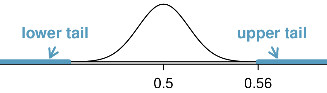
It’s generally helpful to draw null distribution and the tail areas of interest for computing the p-value, as shown in FigureΒ 5.3.21. The upper tail area is about 0.0001, and we double this tail area to get the p-value: 0.0002.
Because the p-value is smaller than 0.05, we reject \(H_0\text{.}\) The poll provides convincing evidence that a majority of Americans supported nuclear arms reduction efforts in March 2013.
Normal distribution centered at 0.5 showing tail areas for nuclear arms test
Figure 5.3.21. A normal distribution centered at 0.5 is shown, which has a standard deviation of about 0.0156. Two tails several standard deviations away from the center are emphasized. The first, at and above 0.56, is annotated with the text "upper tail". The second, which appears to be at and below 0.44, is annotated with the text "lower tail".

Hypothesis testing for a single proportion.

Once you’ve determined a one-proportion hypothesis test is the correct procedure, there are four steps to completing the test:
Prepare.
Identify the parameter of interest, list hypotheses, identify the significance level, and identify \(\hat{p}\) and \(n\text{.}\)
Check.
Verify conditions to ensure \(\hat{p}\) is nearly normal under \(H_0\text{.}\) For one-proportion hypothesis tests, use the null value to check the success-failure condition.
Calculate.
If the conditions hold, compute the standard error, again using \(p_0\text{,}\) compute the Z-score, and identify the p-value.
Conclude.
Evaluate the hypothesis test by comparing the p-value to \(\alpha\text{,}\) and provide a conclusion in the context of the problem.

Subsection 5.3.5 Choosing a Significance Level

Choosing a significance level for a test is important in many contexts, and the traditional level is \(\alpha = 0.05\text{.}\) However, it can be helpful to adjust the significance level based on the application. We may select a level that is smaller or larger than 0.05 depending on the consequences of any conclusions reached from the test.
If making a Type 1 Error is dangerous or especially costly, we should choose a small significance level (e.g. 0.01). Under this scenario we want to be very cautious about rejecting the null hypothesis, so we demand very strong evidence favoring \(H_A\) before we would reject \(H_0\text{.}\)
If a Type 2 Error is relatively more dangerous or much more costly than a Type 1 Error, then we might choose a higher significance level (e.g. 0.10). Here we want to be cautious about failing to reject \(H_0\) when the alternative hypothesis is actually true.
Additionally, if the cost of collecting data is small relative to the cost of a Type 2 Error, then it may also be a good strategy to collect more data. Under this strategy, the Type 2 Error can be reduced while not affecting the Type 1 Error rate. Of course, collecting extra data is often costly, so there is typically a cost-benefit analysis to be considered.

Subsection 5.3.6 Statistical Significance versus Practical Significance

When the sample size becomes larger, point estimates become more precise and any real differences in the mean and null value become easier to detect and recognize. Even a very small difference would likely be detected if we took a large enough sample. Sometimes researchers will take such large samples that even the slightest difference is detected, even differences where there is no practical value. In such cases, we still say the difference is statistically significant, but it is not practically significant.
For example, an online experiment might identify that placing additional ads on a movie review website statistically significantly increases viewership of a TV show by 0.001%, but this increase might not have any practical value.
One role of a data scientist in conducting a study often includes planning the size of the study. The data scientist might first consult experts or scientific literature to learn what would be the smallest meaningful difference from the null value. She also would obtain other information, such as a very rough estimate of the true proportion \(p\text{,}\) so that she could roughly estimate the standard error. From here, she can suggest a sample size that is sufficiently large that, if there is a real difference that is meaningful, we could detect it. While larger sample sizes may still be used, these calculations are especially helpful when considering costs or potential risks, such as possible health impacts to volunteers in a medical study.

Subsection 5.3.7 One-Sided Hypothesis Tests (Special Topic)

So far we’ve only considered what are called two-sided hypothesis tests, where we care about detecting whether \(p\) is either above or below some null value \(p_0\text{.}\) There is a second type of hypothesis test called a one-sided hypothesis test.
For a one-sided hypothesis test, the hypotheses take one of the following forms:
  1. There’s only value in detecting if the population parameter is less than some value \(p_0\text{.}\) In this case, the alternative hypothesis is written as \(p < p_0\) for some null value \(p_0\text{.}\)
  2. There’s only value in detecting if the population parameter is more than some value \(p_0\text{:}\) In this case, the alternative hypothesis is written as \(p > p_0\text{.}\)
While we adjust the form of the alternative hypothesis, we continue to write the null hypothesis using an equals-sign in the one-sided hypothesis test case.
In the entire hypothesis testing procedure, there is only one difference in evaluating a one-sided hypothesis test vs a two-sided hypothesis test: how to compute the p-value. In a one-sided hypothesis test, we compute the p-value as the tail area in the direction of the alternative hypothesis only, meaning it is represented by a single tail area. Herein lies the reason why one-sided tests are sometimes interesting: if we don’t have to double the tail area to get the p-value, then the p-value is smaller and the level of evidence required to identify an interesting finding in the direction of the alternative hypothesis goes down. However, one-sided tests aren’t all sunshine and rainbows: the heavy price paid is that any interesting findings in the opposite direction must be disregarded.

Example 5.3.22.

In SubsectionΒ 5.3.1, we encountered an example where doctors were interested in determining whether stents would help people who had a high risk of stroke. The researchers believed the stents would help. Unfortunately, the data showed the opposite: patients who received stents actually did worse. Why was using a two-sided test so important in this context?
Solution.
Before the study, researchers had reason to believe that stents would help patients since existing research suggested stents helped in patients with heart attacks. It would surely have been tempting to use a one-sided test in this situation, and had they done this, they would have limited their ability to identify potential harm to patients.
This example highlights that using a one-sided hypothesis creates a risk of overlooking data supporting the opposite conclusion. We could have made a similar error when reviewing the Roslings’ question data in this section; if we had a pre-conceived notion that college-educated people wouldn’t do worse than random guessing and so used a one-sided test, we would have missed the really interesting finding that many people have incorrect knowledge about global public health.
When might a one-sided test be appropriate to use? Very rarely. Should you ever find yourself considering using a one-sided test, carefully answer the following question:
What would I, or others, conclude if the data happens to go clearly in the opposite direction than my alternative hypothesis?
If you or others would find any value in making a conclusion about the data that goes in the opposite direction of a one-sided test, then a two-sided hypothesis test should actually be used. These considerations can be subtle, so exercise caution. We will only apply two-sided tests in the rest of this book.

Example 5.3.23.

Why can’t we simply run a one-sided test that goes in the direction of the data?
Solution.
We’ve been building a careful framework that controls for the Type 1 Error, which is the significance level \(\alpha\) in a hypothesis test. We’ll use the \(\alpha = 0.05\) below to keep things simple.
Imagine we could pick the one-sided test after we saw the data. What will go wrong?
  • If \(\hat{p}\) is smaller than the null value, then a one-sided test where \(p < p_0\) would mean that any observation in the lower 5% tail of the null distribution would lead to us rejecting \(H_0\text{.}\)
  • If \(\hat{p}\) is larger than the null value, then a one-sided test where \(p > p_0\) would mean that any observation in the upper 5% tail of the null distribution would lead to us rejecting \(H_0\text{.}\)
Then if \(H_0\) were true, there’s a 10% chance of being in one of the two tails, so our testing error is actually \(\alpha = 0.10\text{,}\) not 0.05. That is, not being careful about when to use one-sided tests effectively undermines the methods we’re working so hard to develop and utilize.

Warning 5.3.24.

Use one-sided tests only when you have a strong reason to care about deviations in only one direction. If you’re unsure, use a two-sided test.

Exercises 5.3.8 Section 5.3 Exercises

1. Identify hypotheses, Part I..

Write the null and alternative hypotheses in words and then symbols for each of the following situations.
  1. A tutoring company would like to understand if most students tend to improve their grades (or not) after they use their services. They sample 200 of the students who used their service in the past year and ask them if their grades have improved or declined from the previous year.
  2. Employers at a firm are worried about the effect of March Madness, a basketball championship held each spring in the US, on employee productivity. They estimate that on a regular business day employees spend on average 15 minutes of company time checking personal email, making personal phone calls, etc. They also collect data on how much company time employees spend on such non-business activities during March Madness. They want to determine if these data provide convincing evidence that employee productivity changed during March Madness.

2. Identify hypotheses, Part II..

Write the null and alternative hypotheses in words and using symbols for each of the following situations.
  1. Since 2008, chain restaurants in California have been required to display calorie counts of each menu item. Prior to menus displaying calorie counts, the average calorie intake of diners at a restaurant was 1100 calories. After calorie counts started to be displayed on menus, a nutritionist collected data on the number of calories consumed at this restaurant from a random sample of diners. Do these data provide convincing evidence of a difference in the average calorie intake of diners at this restaurant?
  2. The state of Wisconsin would like to understand the fraction of its adult residents that consumed alcohol in the last year, specifically if the rate is different from the national rate of 70%. To help them answer this question, they conduct a random sample of 852 residents and ask them about their alcohol consumption.

3. Online communication..

A study suggests that 60% of college students spend 10 or more hours per week communicating with others online. You believe that this is incorrect and decide to collect your own sample for a hypothesis test. You randomly sample 160 students from your dorm and find that 70% spent 10 or more hours a week communicating with others online. A friend of yours, who offers to help you with the hypothesis test, comes up with the following set of hypotheses. Indicate any errors you see.
\begin{align*} H_0: \amp\ \hat{p} < 0.6\\ H_A: \amp\ \hat{p} > 0.7 \end{align*}

4. Married at 25..

A study suggests that 25% of 25 year olds have gotten married. You believe that this is incorrect and decide to collect your own sample for a hypothesis test. From a random sample of 25 year olds in census data with size 776, you find that 24% of them are married. A friend of yours offers to help you with setting up the hypothesis test and comes up with the following hypotheses. Indicate any errors you see.
\begin{align*} H_0: \amp\ \hat{p} = 0.24\\ H_A: \amp\ \hat{p} \neq 0.24 \end{align*}

5. Cyberbullying rates..

Teens were surveyed about cyberbullying, and 54% to 64% reported experiencing cyberbullying (95% confidence interval). Answer the following questions based on this interval.
  1. A newspaper claims that a majority of teens have experienced cyberbullying. Is this claim supported by the confidence interval? Explain your reasoning.
  2. A researcher conjectured that 70% of teens have experienced cyberbullying. Is this claim supported by the confidence interval? Explain your reasoning.
  3. Without actually calculating the interval, determine if the claim of the researcher from part (b) would be supported based on a 90% confidence interval?

6. Waiting at an ER, Part II..

The ER wait time exercise provides a 95% confidence interval for the mean waiting time at an emergency room (ER) of (128 minutes, 147 minutes). Answer the following questions based on this interval.
  1. A local newspaper claims that the average waiting time at this ER exceeds 3 hours. Is this claim supported by the confidence interval? Explain your reasoning.
  2. The Dean of Medicine at this hospital claims the average wait time is 2.2 hours. Is this claim supported by the confidence interval? Explain your reasoning.
  3. Without actually calculating the interval, determine if the claim of the Dean from part (b) would be supported based on a 99% confidence interval?

7. Minimum wage, Part I..

Do a majority of US adults believe raising the minimum wage will help the economy, or is there a majority who do not believe this? A Rasmussen Reports survey of a random sample of 1,000 US adults found that 42% believe it will help the economy. Conduct an appropriate hypothesis test to help answer the research question.

8. Getting enough sleep..

400 students were randomly sampled from a large university, and 289 said they did not get enough sleep. Conduct a hypothesis test to check whether this represents a statistically significant difference from 50%, and use a significance level of 0.01.

9. Working backwards, Part I..

You are given the following hypotheses:
\begin{align*} H_0: \amp\ p = 0.3\\ H_A: \amp\ p \neq 0.3 \end{align*}
We know the sample size is 90. For what sample proportion would the p-value be equal to 0.05? Assume that all conditions necessary for inference are satisfied.

10. Working backwards, Part II..

You are given the following hypotheses:
\begin{align*} H_0: \amp\ p = 0.9\\ H_A: \amp\ p \neq 0.9 \end{align*}
We know that the sample size is 1,429. For what sample proportion would the p-value be equal to 0.01? Assume that all conditions necessary for inference are satisfied.

11. Testing for Fibromyalgia..

A patient named Diana was diagnosed with Fibromyalgia, a long-term syndrome of body pain, and was prescribed anti-depressants. Being the skeptic that she is, Diana didn’t initially believe that anti-depressants would help her symptoms. However after a couple months of being on the medication she decides that the anti-depressants are working, because she feels like her symptoms are in fact getting better.
  1. Write the hypotheses in words for Diana’s skeptical position when she started taking the anti-depressants.
  2. What is a Type 1 Error in this context?
  3. What is a Type 2 Error in this context?

12. Which is higher?

In each part below, there is a value of interest and two scenarios (I and II). For each part, report if the value of interest is larger under scenario I, scenario II, or whether the value is equal under the scenarios.
  1. The standard error of \(\hat{p}\) when (I) \(n = 125\) or (II) \(n = 500\text{.}\)
  2. The margin of error of a confidence interval when the confidence level is (I) 90% or (II) 80%.
  3. The p-value for a Z-statistic of 2.5 calculated based on a (I) sample with \(n = 500\) or based on a (II) sample with \(n = 1000\text{.}\)
  4. The probability of making a Type 2 Error when the alternative hypothesis is true and the significance level is (I) 0.05 or (II) 0.10.