Difference of two proportions

Section 6.2 Difference of two proportions

We would like to extend the methods from Section 6.1 to apply confidence intervals and hypothesis tests to differences in population proportions: $p_1 - p_2\text{.}$ In our investigations, we’ll identify a reasonable point estimate of $p_1 - p_2$ based on the sample, and you may have already guessed its form: $\hat{p}_1 - \hat{p}_2\text{.}$ Next, we’ll apply the same processes we used in the single-proportion context: we verify that the point estimate can be modeled using a normal distribution, we compute the estimate’s standard error, and we apply our inferential framework.

🔗

Subsection 6.2.1 Sampling distribution of the difference of two proportions

Like with $\hat{p}\text{,}$ the difference of two sample proportions $\hat{p}_1 - \hat{p}_2$ can be modeled using a normal distribution when certain conditions are met. First, we require a broader independence condition, and secondly, the success-failure condition must be met by both groups.

🔗

Conditions for the sampling distribution of $\hat{p}_1 - \hat{p}_2$ to be normal.

The difference $\hat{p}_1 - \hat{p}_2$ can be modeled using a normal distribution when

🔗

When these conditions are satisfied, the standard error of $\hat{p}_1 - \hat{p}_2$ is

🔗

where $p_1$ and $p_2$ represent the population proportions, and $n_1$ and $n_2$ represent the sample sizes.

🔗

Subsection 6.2.2 Confidence intervals for $p_1 - p_2$

We can apply the generic confidence interval formula for a difference of two proportions, where we use $\hat{p}_1 - \hat{p}_2$ as the point estimate and substitute the $SE$ formula:

🔗

\begin{align*} \text{point estimate} \pm z^{\star} \times SE \amp \to \hat{p}_1 - \hat{p}_2 \pm z^{\star} \times \sqrt{\frac{p_1(1-p_1)}{n_1} + \frac{p_2(1-p_2)}{n_2}} \end{align*}

We can also follow the same Prepare, Check, Calculate, Conclude steps for computing a confidence interval or completing a hypothesis test. The details change a little, but the general approach remain the same. Think about these steps when you apply statistical methods.

🔗

Example 6.2.1.

We consider an experiment for patients who underwent cardiopulmonary resuscitation (CPR) for a heart attack and were subsequently admitted to a hospital. These patients were randomly divided into a treatment group where they received a blood thinner or the control group where they did not receive a blood thinner. The outcome variable of interest was whether the patients survived for at least 24 hours. The results are shown in Table 6.2.2. Check whether we can model the difference in sample proportions using the normal distribution.

🔗

Solution.

We first check for independence: since this is a randomized experiment, this condition is satisfied.

🔗

Next, we check the success-failure condition for each group. We have at least 10 successes and 10 failures in each experiment arm (11, 14, 39, 26), so this condition is also satisfied.

🔗

With both conditions satisfied, the difference in sample proportions can be reasonably modeled using a normal distribution for these data.

🔗

Table 6.2.2. Results for the CPR study. Patients in the treatment group were given a blood thinner, and patients in the control group were not.

🔗

	Survived	Died	Total
Control	11	39	50
Treatment	14	26	40
Total	25	65	90

Example 6.2.3.

Create and interpret a 90% confidence interval of the difference for the survival rates in the CPR study.

🔗

Solution.

We’ll use $p_t$ for the survival rate in the treatment group and $p_c$ for the control group:

🔗

\begin{gather*} \hat{p}_{t} - \hat{p}_{c} = \frac{14}{40} - \frac{11}{50} = 0.35 - 0.22 = 0.13 \end{gather*}

We use the standard error formula provided in Assemblage . As with the one-sample proportion case, we use the sample estimates of each proportion in the formula in the confidence interval context:

🔗

\begin{gather*} SE \approx \sqrt{\frac{0.35 (1 - 0.35)}{40} + \frac{0.22 (1 - 0.22)}{50}} = 0.095 \end{gather*}

For a 90% confidence interval, we use $z^{\star} = 1.6449\text{:}$

🔗

\begin{align*} \text{point estimate} \pm z^{\star} \times SE \amp \to 0.13 \pm 1.6449 \times 0.095\\ \amp \to (-0.026, 0.286) \end{align*}

We are 90% confident that blood thinners have a difference of -2.6% to +28.6% percentage point impact on survival rate for patients who are like those in the study. Because 0% is contained in the interval, we do not have enough information to say whether blood thinners help or harm heart attack patients who have been admitted after they have undergone CPR.

🔗

Checkpoint 6.2.4.

A 5-year experiment was conducted to evaluate the effectiveness of fish oils on reducing cardiovascular events, where each subject was randomized into one of two treatment groups. We’ll consider heart attack outcomes in these patients:

🔗

Table 6.2.5.

🔗

	heart attack	no event	Total
fish oil	145	12788	12933
placebo	200	12738	12938

Create a 95% confidence interval for the effect of fish oils on heart attacks for patients who are well-represented by those in the study. Also interpret the interval in the context of the study.

🔗

Solution.

Because the patients were randomized, the subjects are independent, both within and between the two groups. The success-failure condition is also met for both groups as all counts are at least 10. This satisfies the conditions necessary to model the difference in proportions using a normal distribution.

🔗

Compute the sample proportions ($\hat{p}_{\text{fish oil}} = 0.0112\text{,}$ $\hat{p}_{\text{placebo}} = 0.0155$), point estimate of the difference ($0.0112 - 0.0155 = -0.0043$), and standard error ($SE = \sqrt{\frac{0.0112 \times 0.9888}{12933} + \frac{0.0155 \times 0.9845}{12938}} = 0.00145$). Next, plug the values into the general formula for a confidence interval, where we’ll use a 95% confidence level with $z^{\star} = 1.96\text{:}$

🔗

\begin{gather*} -0.0043 \pm 1.96 \times 0.00145 \to (-0.0071, -0.0015) \end{gather*}

We are 95% confident that fish oils decreases heart attacks by 0.15 to 0.71 percentage points (off of a baseline of about 1.55%) over a 5-year period for subjects who are similar to those in the study. Because the interval is entirely below 0, the data provide strong evidence that fish oil supplements reduce heart attacks in patients like those in the study.

🔗

Subsection 6.2.3 Hypothesis tests for the difference of two proportions

A mammogram is an X-ray procedure used to check for breast cancer. Whether mammograms should be used is part of a controversial discussion, and it’s the topic of our next example where we learn about 2-proportion hypothesis tests when $H_0$ is $p_1 - p_2 = 0$ (or equivalently, $p_1 = p_2$).

🔗

A 30-year study was conducted with nearly 90,000 female participants. During a 5-year screening period, each woman was randomized to one of two groups: in the first group, women received regular mammograms to screen for breast cancer, and in the second group, women received regular non-mammogram breast cancer exams. No intervention was made during the following 25 years of the study, and we’ll consider death resulting from breast cancer over the full 30-year period. Results from the study are summarized in Table 6.2.6.

🔗

If mammograms are much more effective than non-mammogram breast cancer exams, then we would expect to see additional deaths from breast cancer in the control group. On the other hand, if mammograms are not as effective as regular breast cancer exams, we would expect to see an increase in breast cancer deaths in the mammogram group.

🔗

Table 6.2.6. Summary results for breast cancer study.

🔗

	Death from breast cancer?
	Yes	No
Mammogram	500	44,425
Control	505	44,405

Checkpoint 6.2.7.

Is this study an experiment or an observational study?

🔗

Solution.

This is an experiment. Patients were randomized to receive mammograms or a standard breast cancer exam. We will be able to make causal conclusions based on this study.

🔗

Checkpoint 6.2.8.

Set up hypotheses to test whether there was a difference in breast cancer deaths in the mammogram and control groups.

🔗

Solution.

$H_0\text{:}$ the breast cancer death rate for patients screened using mammograms is the same as the breast cancer death rate for patients in the control, $p_{mgm} - p_{ctrl} = 0\text{.}$

🔗

$H_A\text{:}$ the breast cancer death rate for patients screened using mammograms is different than the breast cancer death rate for patients in the control, $p_{mgm} - p_{ctrl} \neq 0\text{.}$

🔗

In Example 6.2.9, we will check the conditions for using a normal distribution to analyze the results of the study. The details are very similar to that of confidence intervals. However, when the null hypothesis is that $p_1 - p_2 = 0\text{,}$ we use a special proportion called the pooled proportion to check the success-failure condition:

🔗

\begin{align*} \hat{p}_{\textit{pooled}} \amp = \frac{\text{\# of patients who died from breast cancer in the entire study}}{\text{\# of patients in the entire study}}\\ \amp = \frac{500 + 505}{500 + \text{44,425} + 505 + \text{44,405}}\\ \amp = 0.0112 \end{align*}

This proportion is an estimate of the breast cancer death rate across the entire study, and it’s our best estimate of the proportions $p_{mgm}$ and $p_{ctrl}$ if the null hypothesis is true that $p_{mgm} = p_{ctrl}$. We will also use this pooled proportion when computing the standard error.

🔗

Example 6.2.9.

Is it reasonable to model the difference in proportions using a normal distribution in this study?

🔗

Solution.

Because the patients are randomized, they can be treated as independent, both within and between groups. We also must check the success-failure condition for each group. Under the null hypothesis, the proportions $p_{mgm}$ and $p_{ctrl}$ are equal, so we check the success-failure condition with our best estimate of these values under $H_0\text{,}$ the pooled proportion from the two samples, $\hat{p}_{\textit{pooled}} = 0.0112\text{:}$

🔗

\begin{align*} \hat{p}_{\textit{pooled}} \times n_{mgm} \amp = 0.0112 \times \text{44,925} = 503\\ (1 - \hat{p}_{\textit{pooled}}) \times n_{mgm} \amp = 0.9888 \times \text{44,925} = \text{44,422}\\ \hat{p}_{\textit{pooled}} \times n_{ctrl} \amp = 0.0112 \times \text{44,910} = 503\\ (1 - \hat{p}_{\textit{pooled}}) \times n_{ctrl} \amp = 0.9888 \times \text{44,910} = \text{44,407} \end{align*}

The success-failure condition is satisfied since all values are at least 10. With both conditions satisfied, we can safely model the difference in proportions using a normal distribution.

🔗

Use the pooled proportion when $H_0$ is $p_1 - p_2 = 0$.

When the null hypothesis is that the proportions are equal, use the pooled proportion ($\hat{p}_{\textit{pooled}}$) to verify the success-failure condition and estimate the standard error:

🔗

Here $\hat{p}_1 n_1$ represents the number of successes in sample 1 since

🔗

Similarly, $\hat{p}_2 n_2$ represents the number of successes in sample 2.

🔗

In Example 6.2.9, the pooled proportion was used to check the success-failure condition.

For an example of a two-proportion hypothesis test that does not require the success-failure condition to be met, see Section 2.3.

In the next example, we see the second place where the pooled proportion comes into play: the standard error calculation.

🔗

Example 6.2.10.

Compute the point estimate of the difference in breast cancer death rates in the two groups, and use the pooled proportion $\hat{p}_{\textit{pooled}} = 0.0112$ to calculate the standard error.

🔗

Solution.

The point estimate of the difference in breast cancer death rates is

🔗

\begin{align*} \hat{p}_{mgm} - \hat{p}_{ctrl} \amp = \frac{500}{500 + 44,425} - \frac{505}{505 + 44,405}\\ \amp = 0.01113 - 0.01125\\ \amp = -0.00012 \end{align*}

The breast cancer death rate in the mammogram group was 0.012% less than in the control group. Next, the standard error is calculated using the pooled proportion, $\hat{p}_{\textit{pooled}}\text{:}$

🔗

\begin{gather*} SE = \sqrt{\frac{\hat{p}_{\textit{pooled}}(1-\hat{p}_{\textit{pooled}})}{n_{mgm}} + \frac{\hat{p}_{\textit{pooled}}(1-\hat{p}_{\textit{pooled}})}{n_{ctrl}}} = 0.00070 \end{gather*}

🔗

Example 6.2.11.

Using the point estimate $\hat{p}_{mgm} - \hat{p}_{ctrl} = -0.00012$ and standard error $SE = 0.00070\text{,}$ calculate a p-value for the hypothesis test and write a conclusion.

🔗

Solution.

Just like in past tests, we first compute a test statistic and draw a picture:

🔗

\begin{gather*} Z = \frac{\text{point estimate} - \text{null value}}{SE} = \frac{-0.00012 - 0}{0.00070} = -0.17 \end{gather*}

Figure 6.2.12. A normal distribution is shown centered at 0 with a standard deviation of 0.0007. The lower tail is shaded below -0.00012 and the upper tail is shaded above 0.00012. Visually, it looks like very roughly 90% of the area under the normal distribution is shaded.
🔗

The lower tail area is 0.4325, which we double to get the p-value: 0.8650. Because this p-value is larger than 0.05, we do not reject the null hypothesis. That is, the difference in breast cancer death rates is reasonably explained by chance, and we do not observe benefits or harm from mammograms relative to a regular breast exam.

🔗

Can we conclude that mammograms have no benefits or harm? Here are a few considerations to keep in mind when reviewing the mammogram study as well as any other medical study:

🔗

We do not reject the null hypothesis, which means we don’t have sufficient evidence to conclude that mammograms reduce or increase breast cancer deaths.

🔗
If mammograms are helpful or harmful, the data suggest the effect isn’t very large.

🔗
Are mammograms more or less expensive than a non-mammogram breast exam? If one option is much more expensive than the other and doesn’t offer clear benefits, then we should lean towards the less expensive option.

🔗
The study’s authors also found that mammograms led to overdiagnosis of breast cancer, which means some breast cancers were found (or thought to be found) but that these cancers would not cause symptoms during patients’ lifetimes. That is, something else would kill the patient before breast cancer symptoms appeared. This means some patients may have been treated for breast cancer unnecessarily, and this treatment is another cost to consider. It is also important to recognize that overdiagnosis can cause unnecessary physical or emotional harm to patients.

🔗

These considerations highlight the complexity around medical care and treatment recommendations. Experts and medical boards who study medical treatments use considerations like those above to provide their best recommendation based on the current evidence.

🔗

Subsection 6.2.4 More on 2-proportion hypothesis tests (special topic)

When we conduct a 2-proportion hypothesis test, usually $H_0$ is $p_1 - p_2 = 0\text{.}$ However, there are rare situations where we want to check for some difference in $p_1$ and $p_2$ that is some value other than 0. For example, maybe we care about checking a null hypothesis where $p_1 - p_2 = 0.1\text{.}$ In contexts like these, we generally use $\hat{p}_1$ and $\hat{p}_2$ to check the success-failure condition and construct the standard error.

🔗

Checkpoint 6.2.13.

A quadcopter company is considering a new manufacturer for rotor blades. The new manufacturer would be more expensive, but they claim their higher-quality blades are more reliable, with 3% more blades passing inspection than their competitor. Set up appropriate hypotheses for the test.

🔗

Solution.

$H_0\text{:}$ The higher-quality blades will pass inspection 3% more frequently than the standard-quality blades. $p_{highQ} - p_{standard} = 0.03\text{.}$

🔗

$H_A\text{:}$ The higher-quality blades will pass inspection some amount different than 3% more often than the standard-quality blades. $p_{highQ} - p_{standard} \neq 0.03\text{.}$

🔗

Figure 6.2.14. A Phantom quadcopter. Photo by David J (http://flic.kr/p/oiWLNu). CC-BY 2.0 license. This photo has been cropped and a border has been added.
🔗

Example 6.2.15.

The quality control engineer from Checkpoint 6.2.13 collects a sample of blades, examining 1000 blades from each company, and she finds that 899 blades pass inspection from the current supplier and 958 pass inspection from the prospective supplier. Using these data, evaluate the hypotheses from Checkpoint 6.2.13 with a significance level of 5%.

🔗

Solution.

First, we check the conditions. The sample is not necessarily random, so to proceed we must assume the blades are all independent; for this sample we will suppose this assumption is reasonable, but the engineer would be more knowledgeable as to whether this assumption is appropriate. The success-failure condition also holds for each sample. Thus, the difference in sample proportions, $0.958 - 0.899 = 0.059\text{,}$ can be said to come from a nearly normal distribution.

🔗

The standard error is computed using the two sample proportions since we do not use a pooled proportion for this context:

🔗

\begin{gather*} SE = \sqrt{\frac{0.958(1-0.958)}{1000} + \frac{0.899(1-0.899)}{1000}} = 0.0114 \end{gather*}

In this hypothesis test, because the null is that $p_1 - p_2 = 0.03\text{,}$ the sample proportions were used for the standard error calculation rather than a pooled proportion.

🔗

Next, we compute the test statistic and use it to find the p-value, which is depicted in Figure 6.2.16.

🔗

\begin{gather*} Z = \frac{\text{point estimate} - \text{null value}}{SE} = \frac{0.059 - 0.03}{0.0114} = 2.54 \end{gather*}

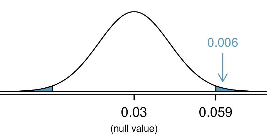
Using a standard normal distribution for this test statistic, we identify the right tail area as 0.006, and we double it to get the p-value: 0.012. We reject the null hypothesis because 0.012 is less than 0.05. Since we observed a larger-than-3% increase in blades that pass inspection, we have statistically significant evidence that the higher-quality blades pass inspection more than 3% as often as the currently used blades, exceeding the company’s claims.

🔗

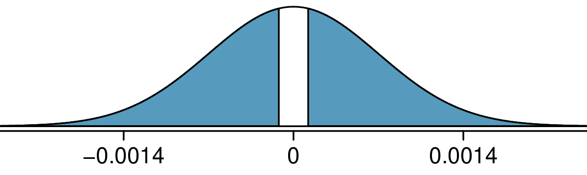
Figure 6.2.16. Distribution of the test statistic if the null hypothesis was true. The p-value is represented by the shaded areas.
🔗

🔗

Subsection 6.2.5 Examining the standard error formula (special topic)

This subsection covers more theoretical topics that offer deeper insights into the origins of the standard error formula for the difference of two proportions. Ultimately, all of the standard error formulas we encounter in this chapter and in Chapter 7 can be derived from the probability principles of Section 3.4.

🔗

The formula for the standard error of the difference in two proportions can be deconstructed into the formulas for the standard errors of the individual sample proportions. Recall that the standard error of the individual sample proportions $\hat{p}_1$ and $\hat{p}_2$ are

🔗

\begin{gather*} SE_{\hat{p}_1} = \sqrt{\frac{{p}_1 (1 - {p}_1)}{n_1}} \qquad SE_{\hat{p}_2} = \sqrt{\frac{{p}_2 (1 - {p}_2)}{n_2}} \end{gather*}

The standard error of the difference of two sample proportions can be deconstructed from the standard errors of the separate sample proportions:

🔗

\begin{gather*} SE_{\hat{p}_{1} - \hat{p}_{2}} = \sqrt{SE_{\hat{p}_1}^2 + SE_{\hat{p}_2}^2} = \sqrt{\frac{{p}_1 (1 - {p}_1)}{n_1} + \frac{{p}_2 (1 - {p}_2)}{n_2}} \end{gather*}

This special relationship follows from probability theory.

🔗

Checkpoint 6.2.17.

Prerequisite: Section 3.4. We can rewrite the equation above in a different way:

🔗

\begin{equation*} SE_{\hat{p}_{1} - \hat{p}_{2}}^2 = SE_{\hat{p}_1}^2 + SE_{\hat{p}_2}^2 \end{equation*}

Explain where this formula comes from using the formula for the variability of the sum of two random variables.

🔗

Solution.

The standard error squared represents the variance of the estimate. If $X$ and $Y$ are two random variables with variances $\sigma_x^2$ and $\sigma_y^2\text{,}$ then the variance of $X - Y$ is $\sigma_x^2 + \sigma_y^2\text{.}$ Likewise, the variance corresponding to $\hat{p}_1 - \hat{p}_2$ is $\sigma_{\hat{p}_1}^2 + \sigma_{\hat{p}_2}^2\text{.}$ Because $\sigma_{\hat{p}_1}^2$ and $\sigma_{\hat{p}_2}^2$ are just another way of writing $SE_{\hat{p}_1}^2$ and $SE_{\hat{p}_2}^2\text{,}$ the variance associated with $\hat{p}_1 - \hat{p}_2$ may be written as $SE_{\hat{p}_1}^2 + SE_{\hat{p}_2}^2\text{.}$

🔗

Exercises 6.2.6 Section 6.2 Exercises

1. Social experiment, Part I.

A "social experiment" conducted by a TV program questioned what people do when they see a very obviously bruised woman getting picked on by her boyfriend. On two different occasions at the same restaurant, the same couple was depicted. In one scenario the woman was dressed "provocatively" and in the other scenario the woman was dressed "conservatively". The table below shows how many restaurant diners were present under each scenario, and whether or not they intervened.

🔗

		Scenario
		Provocative	Conservative	Total
Intervene	Yes	5	15	20
	No	15	10	25
	Total	20	25	45

Explain why the sampling distribution of the difference between the proportions of interventions under provocative and conservative scenarios does not follow an approximately normal distribution.

🔗

2. Heart transplant success.

The Stanford University Heart Transplant Study was conducted to determine whether an experimental heart transplant program increased lifespan. Each patient entering the program was officially designated a heart transplant candidate, meaning that he was gravely ill and might benefit from a new heart. Patients were randomly assigned into treatment and control groups. Patients in the treatment group received a transplant, and those in the control group did not. The table below displays how many patients survived and died in each group.

🔗

	control	treatment
alive	4	24
dead	30	45

Suppose we are interested in estimating the difference in survival rate between the control and treatment groups using a confidence interval. Explain why we cannot construct such an interval using the normal approximation. What might go wrong if we constructed the confidence interval despite this problem?

🔗

3. Gender and color preference.

A study asked 1,924 male and 3,666 female undergraduate college students their favorite color. A 95% confidence interval for the difference between the proportions of males and females whose favorite color is black $(p_{male} - p_{female})$ was calculated to be (0.02, 0.06). Based on this information, determine if the following statements about undergraduate college students are true or false, and explain your reasoning for each statement you identify as false.

🔗

We are 95% confident that the true proportion of males whose favorite color is black is 2% lower to 6% higher than the true proportion of females whose favorite color is black.

🔗
We are 95% confident that the true proportion of males whose favorite color is black is 2% to 6% higher than the true proportion of females whose favorite color is black.

🔗
95% of random samples will produce 95% confidence intervals that include the true difference between the population proportions of males and females whose favorite color is black.

🔗
We can conclude that there is a significant difference between the proportions of males and females whose favorite color is black and that the difference between the two sample proportions is too large to plausibly be due to chance.

🔗
The 95% confidence interval for $(p_{female} - p_{male})$ cannot be calculated with only the information given in this exercise.

🔗

🔗

4. Government shutdown.

The United States federal government shutdown of 2018–2019 occurred from December 22, 2018 until January 25, 2019, a span of 35 days. A Survey USA poll of 614 randomly sampled Americans during this time period reported that 48% of those who make less than $40,000 per year and 55% of those who make $40,000 or more per year said the government shutdown has not at all affected them personally. A 95% confidence interval for $(p_{\text{$\lt$40K}} - p_{\text{$\ge$40K}})\text{,}$ where $p$ is the proportion of those who said the government shutdown has not at all affected them personally, is (-0.16, 0.02). Based on this information, determine if the following statements are true or false, and explain your reasoning if you identify the statement as false.

🔗

At the 5% significance level, the data provide convincing evidence of a real difference in the proportion who are not affected personally between Americans who make less than $40,000 annually and Americans who make $40,000 annually.

🔗
We are 95% confident that 16% more to 2% fewer Americans who make less than $40,000 per year are not at all personally affected by the government shutdown compared to those who make $40,000 or more per year.

🔗
A 90% confidence interval for $(p_{\text{$\lt$40K}} - p_{\text{$\ge$40K}})$ would be wider than the $(-0.16, 0.02)$ interval.

🔗
A 95% confidence interval for $(p_{\text{$\ge$40K}} - p_{\text{$\lt$40K}})$ is (-0.02, 0.16).

🔗

🔗

5. National Health Plan, Part III.

Exercise 6.1.6.11 presents the results of a poll evaluating support for a generically branded "National Health Plan" in the United States. 79% of 347 Democrats and 55% of 617 Independents support a National Health Plan.

🔗

Calculate a 95% confidence interval for the difference between the proportion of Democrats and Independents who support a National Health Plan $(p_{D} - p_{I})\text{,}$ and interpret it in this context. We have already checked conditions for you.

🔗
True or false: If we had picked a random Democrat and a random Independent at the time of this poll, it is more likely that the Democrat would support the National Health Plan than the Independent.

🔗

🔗

6. Sleep deprivation, CA vs. OR, Part I.

According to a report on sleep deprivation by the Centers for Disease Control and Prevention, the proportion of California residents who reported insufficient rest or sleep during each of the preceding 30 days is 8.0%, while this proportion is 8.8% for Oregon residents. These data are based on simple random samples of 11,545 California and 4,691 Oregon residents. Calculate a 95% confidence interval for the difference between the proportions of Californians and Oregonians who are sleep deprived and interpret it in context of the data.

🔗

7. Offshore drilling, Part I.

A survey asked 827 randomly sampled registered voters in California "Do you support? Or do you oppose? Drilling for oil and natural gas off the Coast of California? Or do you not know enough to say?" Below is the distribution of responses, separated based on whether or not the respondent graduated from college.

🔗

	College Grad
	Yes	No
Support	154	132
Oppose	180	126
Do not know	104	131
Total	438	389

What percent of college graduates and what percent of the non-college graduates in this sample do not know enough to have an opinion on drilling for oil and natural gas off the Coast of California?

🔗
Conduct a hypothesis test to determine if the data provide strong evidence that the proportion of college graduates who do not have an opinion on this issue is different than that of non-college graduates.

🔗

🔗

8. Sleep deprivation, CA vs. OR, Part II.

Exercise 6.2.6.6 provides data on sleep deprivation rates of Californians and Oregonians. The proportion of California residents who reported insufficient rest or sleep during each of the preceding 30 days is 8.0%, while this proportion is 8.8% for Oregon residents. These data are based on simple random samples of 11,545 California and 4,691 Oregon residents.

🔗

Conduct a hypothesis test to determine if these data provide strong evidence the rate of sleep deprivation is different for the two states. (Reminder: Check conditions)

🔗
It is possible the conclusion of the test in part (a) is incorrect. If this is the case, what type of error was made?

🔗

🔗

9. Offshore drilling, Part II.

Results of a poll evaluating support for drilling for oil and natural gas off the coast of California were introduced in Exercise 6.2.6.7.

🔗

	College Grad
	Yes	No
Support	154	132
Oppose	180	126
Do not know	104	131
Total	438	389

What percent of college graduates and what percent of the non-college graduates in this sample support drilling for oil and natural gas off the Coast of California?

🔗
Conduct a hypothesis test to determine if the data provide strong evidence that the proportion of college graduates who support off-shore drilling in California is different than that of non-college graduates.

🔗

🔗

10. Full body scan, Part I.

A news article reports that "Americans have differing views on two potentially inconvenient and invasive practices that airports could implement to uncover potential terrorist attacks." This news piece was based on a survey conducted among a random sample of 1,137 adults nationwide, where one of the questions on the survey was "Some airports are now using ’full-body’ digital x-ray machines to electronically screen passengers in airport security lines. Do you think these new x-ray machines should or should not be used at airports?" Below is a summary of responses based on party affiliation.

🔗

		Party Affiliation
		Republican	Democrat	Independent
Answer	Should	264	299	351
	Should not	38	55	77
	Don’t know/No answer	16	15	22
	Total	318	369	450

Conduct an appropriate hypothesis test evaluating whether there is a difference in the proportion of Republicans and Democrats who think the full-body scans should be applied in airports. Assume that all relevant conditions are met.

🔗
The conclusion of the test in part (a) may be incorrect, meaning a testing error was made. If an error was made, was it a Type 1 or a Type 2 Error? Explain.

🔗

🔗

11. Sleep deprived transportation workers.

The National Sleep Foundation conducted a survey on the sleep habits of randomly sampled transportation workers and a control sample of non-transportation workers. The results of the survey are shown below.

🔗

		Transportation Professionals
	Control	Pilots	Truck Drivers	Train Operators	Bus/Taxi/Limo Drivers
Less than 6 hours of sleep	35	19	35	29	21
6 to 8 hours of sleep	193	132	117	119	131
More than 8 hours	64	51	51	32	58
Total	292	202	203	180	210

Conduct a hypothesis test to evaluate if these data provide evidence of a difference between the proportions of truck drivers and non-transportation workers (the control group) who get less than 6 hours of sleep per day, i.e. are considered sleep deprived.

🔗

12. Prenatal vitamins and Autism.

Researchers studying the link between prenatal vitamin use and autism surveyed the mothers of a random sample of children aged 24 - 60 months with autism and conducted another separate random sample for children with typical development. The table below shows the number of mothers in each group who did and did not use prenatal vitamins during the three months before pregnancy (periconceptional period).

🔗

		Autism
		Autism	Typical development	Total
Periconceptional	No vitamin	111	70	181
prenatal vitamin	Vitamin	143	159	302
	Total	254	229	483

State appropriate hypotheses to test for independence of use of prenatal vitamins during the three months before pregnancy and autism.

🔗
Complete the hypothesis test and state an appropriate conclusion. (Reminder: Verify any necessary conditions for the test.)

🔗
A New York Times article reporting on this study was titled "Prenatal Vitamins May Ward Off Autism". Do you find the title of this article to be appropriate? Explain your answer. Additionally, propose an alternative title.

🔗

🔗

13. HIV in sub-Saharan Africa.

In July 2008 the US National Institutes of Health announced that it was stopping a clinical study early because of unexpected results. The study population consisted of HIV-infected women in sub-Saharan Africa who had been given single dose Nevaripine (a treatment for HIV) while giving birth, to prevent transmission of HIV to the infant. The study was a randomized comparison of continued treatment of a woman (after successful childbirth) with Nevaripine vs Lopinavir, a second drug used to treat HIV. 240 women participated in the study; 120 were randomized to each of the two treatments. Twenty-four weeks after starting the study treatment, each woman was tested to determine if the HIV infection was becoming worse (an outcome called virologic failure). Twenty-six of the 120 women treated with Nevaripine experienced virologic failure, while 10 of the 120 women treated with the other drug experienced virologic failure.

🔗

Create a two-way table presenting the results of this study.

🔗
State appropriate hypotheses to test for difference in virologic failure rates between treatment groups.

🔗
Complete the hypothesis test and state an appropriate conclusion. (Reminder: Verify any necessary conditions for the test.)

🔗

🔗

14. An apple a day keeps the doctor away.

A physical education teacher at a high school wanting to increase awareness on issues of nutrition and health asked her students at the beginning of the semester whether they believed the expression "an apple a day keeps the doctor away", and 40% of the students responded yes. Throughout the semester she started each class with a brief discussion of a study highlighting positive effects of eating more fruits and vegetables. She conducted the same apple-a-day survey at the end of the semester, and this time 60% of the students responded yes. Can she use a two-proportion method from this section for this analysis? Explain your reasoning.

🔗

Prev Top Next

Introductory Statistics

Section 6.2 Difference of two proportions

Subsection 6.2.1 Sampling distribution of the difference of two proportions

Conditions for the sampling distribution of \(\hat{p}_1 - \hat{p}_2\) to be normal.

Subsection 6.2.2 Confidence intervals for \(p_1 - p_2\)

Example 6.2.1.

Example 6.2.3.

Checkpoint 6.2.4.

Subsection 6.2.3 Hypothesis tests for the difference of two proportions

Checkpoint 6.2.7.

Checkpoint 6.2.8.

Example 6.2.9.

Use the pooled proportion when \(H_0\) is \(p_1 - p_2 = 0\).

Example 6.2.10.

Example 6.2.11.

Subsection 6.2.4 More on 2-proportion hypothesis tests (special topic)

Checkpoint 6.2.13.

Example 6.2.15.

Subsection 6.2.5 Examining the standard error formula (special topic)

Checkpoint 6.2.17.

Exercises 6.2.6 Section 6.2 Exercises

1. Social experiment, Part I.

2. Heart transplant success.

3. Gender and color preference.

4. Government shutdown.

5. National Health Plan, Part III.

6. Sleep deprivation, CA vs. OR, Part I.

7. Offshore drilling, Part I.

8. Sleep deprivation, CA vs. OR, Part II.

9. Offshore drilling, Part II.

10. Full body scan, Part I.

11. Sleep deprived transportation workers.

12. Prenatal vitamins and Autism.

13. HIV in sub-Saharan Africa.

14. An apple a day keeps the doctor away.