Introductory Statistics

Section 7.3 Difference of two means

In this section we consider a difference in two population means, \(\mu_1 - \mu_2\text{,}\) under the condition that the data are not paired. Just as with a single sample, we identify conditions to ensure we can use the \(t\)-distribution with a point estimate of the difference, \(\bar{x}_1 - \bar{x}_2\text{,}\) and a new standard error formula. Other than these two differences, the details are almost identical to the one-mean procedures.
We apply these methods in three contexts: determining whether stem cells can improve heart function, exploring the relationship between pregnant womens’ smoking habits and birth weights of newborns, and exploring whether there is statistically significant evidence that one variation of an exam is harder than another variation. This section is motivated by questions like β€œIs there convincing evidence that newborns from mothers who smoke have a different average birth weight than newborns from mothers who don’t smoke?”

Subsection 7.3.1 Confidence interval for a difference of means

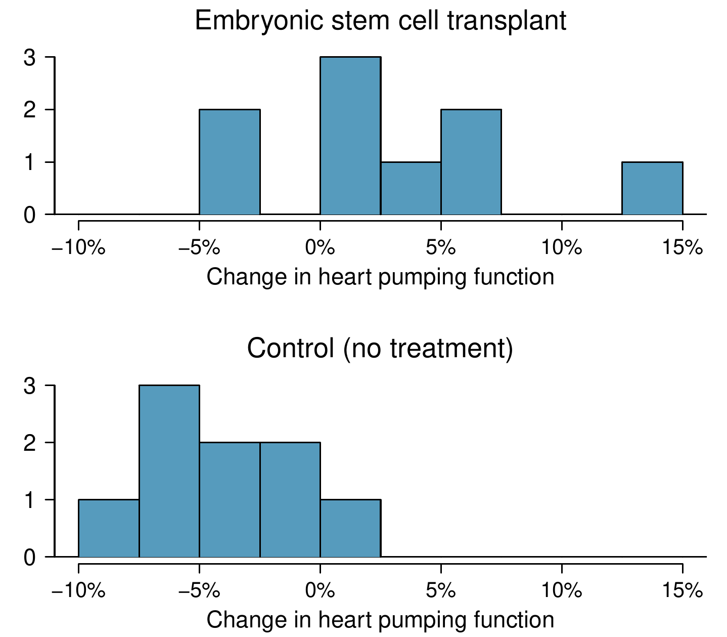
Does treatment using embryonic stem cells (ESCs) help improve heart function following a heart attack? FigureΒ 7.3.1 contains summary statistics for an experiment to test ESCs in sheep that had a heart attack. Each of these sheep was randomly assigned to the ESC or control group, and the change in their hearts’ pumping capacity was measured in the study. FigureΒ 7.3.3 provides histograms of the two data sets. A positive value corresponds to increased pumping capacity, which generally suggests a stronger recovery. Our goal will be to identify a 95% confidence interval for the effect of ESCs on the change in heart pumping capacity relative to the control group.
\(n\) \(\bar{x}\) \(s\)
ESCs 9 3.50 5.17
control 9 \(-4.33\) 2.76
Figure 7.3.1. Summary statistics of the embryonic stem cell study.
The point estimate of the difference in the heart pumping variable is straightforward to find: it is the difference in the sample means.
\begin{align*} \bar{x}_{esc} - \bar{x}_{control} \amp= 3.50 - (-4.33)\\ \amp= 7.83 \end{align*}
For the question of whether we can model this difference using a \(t\)-distribution, we’ll need to check new conditions. Like the 2-proportion cases, we will require a more robust version of independence so we are confident the two groups are also independent. Secondly, we also check for normality in each group separately, which in practice is a check for outliers.

Using the \(t\)-distribution for a difference in means.

The \(t\)-distribution can be used for inference when working with the standardized difference of two means if
The standard error may be computed as
The official formula for the degrees of freedom is quite complex and is generally computed using software, so instead you may use the smaller of \(n_1 - 1\) and \(n_2 - 1\) for the degrees of freedom if software isn’t readily available.
Example 7.3.2.

Can the \(t\)-distribution be used to make inference using the point estimate, \(\bar{x}_{esc} - \bar{x}_{control} = 7.83\text{?}\)
Solution.
First, we check for independence. Because the sheep were randomized into the groups, independence within and between groups is satisfied.
FigureΒ 7.3.3 does not reveal any clear outliers in either group. (The ESC group does look a bit more variability, but this is not the same as having clear outliers.)
With both conditions met, we can use the \(t\)-distribution to model the difference of sample means.
Two histograms are shown, one for "Embryonic stem cell transplant" and one for "Control (no treatment)". The data for the first histogram for the treatment group are roughly centered at about 3%, with values ranging from about -5% to positive 15%. The data for the second histogram, which represents the control group, is approximately centered at -3%, with values ranging from -10% to about positive 2%.
Figure 7.3.3. Histograms for both the embryonic stem cell and control group.
As with the one-sample case, we always compute the standard error using sample standard deviations rather than population standard deviations:
\begin{align*} SE \amp= \sqrt{\frac{s_{esc}^2}{n_{esc}} + \frac{s_{control}^2}{n_{control}}}\\ \amp= \sqrt{\frac{5.17^2}{9} + \frac{2.76^2}{9}}\\ \amp= 1.95 \end{align*}
Generally, we use statistical software to find the appropriate degrees of freedom, or if software isn’t available, we can use the smaller of \(n_1 - 1\) and \(n_2 - 1\) for the degrees of freedom, e.g. if using a \(t\)-table to find tail areas. For transparency in the Examples and Guided Practice, we’ll use the latter approach for finding \(df\text{;}\) in the case of the ESC example, this means we’ll use \(df = 8\text{.}\)

Example 7.3.4.

Calculate a 95% confidence interval for the effect of ESCs on the change in heart pumping capacity of sheep after they’ve suffered a heart attack.
Solution.
We will use the sample difference and the standard error that we computed earlier calculations:
\begin{gather*} \bar{x}_{esc} - \bar{x}_{control} = 7.83 \qquad SE = \sqrt{\frac{5.17^2}{9} + \frac{2.76^2}{9}} = 1.95 \end{gather*}
Using \(df = 8\text{,}\) we can identify the critical value of \(t^{\star}_{8} = 2.31\) for a 95% confidence interval. Finally, we can enter the values into the confidence interval formula:
\begin{align*} \text{point estimate} \pm t^{\star} \times SE \amp\rightarrow 7.83 \pm 2.31\times 1.95\\ \amp\rightarrow (3.32, 12.34) \end{align*}
We are 95% confident that embryonic stem cells improve the heart’s pumping function in sheep that have suffered a heart attack by 3.32% to 12.34%.
As with past statistical inference applications, there is a well-trodden procedure.
Prepare.
Retrieve critical contextual information, and if appropriate, set up hypotheses.
Check.
Ensure the required conditions are reasonably satisfied.
Calculate.
Find the standard error, and then construct a confidence interval, or if conducting a hypothesis test, find a test statistic and p-value.
Conclude.
Interpret the results in the context of the application.
The details change a little from one setting to the next, but this general approach remain the same.

Subsection 7.3.2 Hypothesis tests for the difference of two means

A data set called ncbirths represents a random sample of 150 cases of mothers and their newborns in North Carolina over a year. Four cases from this data set are represented in FigureΒ 7.3.5. We are particularly interested in two variables: weight and smoke. The weight variable represents the weights of the newborns and the smoke variable describes which mothers smoked during pregnancy. We would like to know, is there convincing evidence that newborns from mothers who smoke have a different average birth weight than newborns from mothers who don’t smoke? We will use the North Carolina sample to try to answer this question. The smoking group includes 50 cases and the nonsmoking group contains 100 cases.
fage mage weeks weight sex smoke
1 NA 13 37 5.00 female nonsmoker
2 NA 14 36 5.88 female nonsmoker
3 19 15 41 8.13 male smoker
\(\vdots\) \(\vdots\) \(\vdots\) \(\vdots\) \(\vdots\) \(\vdots\) \(\vdots\)
150 45 50 36 9.25 female nonsmoker
Figure 7.3.5. Four cases from the ncbirths data set. The value β€œNA”, shown for the first two entries of the first variable, indicates that piece of data is missing.

Example 7.3.6.

Set up appropriate hypotheses to evaluate whether there is a relationship between a mother smoking and average birth weight.
Solution.
The null hypothesis represents the case of no difference between the groups.
  • \(H_0\text{:}\) There is no difference in average birth weight for newborns from mothers who did and did not smoke. In statistical notation: \(\mu_{n} - \mu_{s} = 0\text{,}\) where \(\mu_{n}\) represents non-smoking mothers and \(\mu_s\) represents mothers who smoked.
  • \(H_A\text{:}\) There is some difference in average newborn weights from mothers who did and did not smoke (\(\mu_{n} - \mu_{s} \neq 0\)).
We check the two conditions necessary to model the difference in sample means using the \(t\)-distribution.
  • Because the data come from a simple random sample, the observations are independent, both within and between samples.
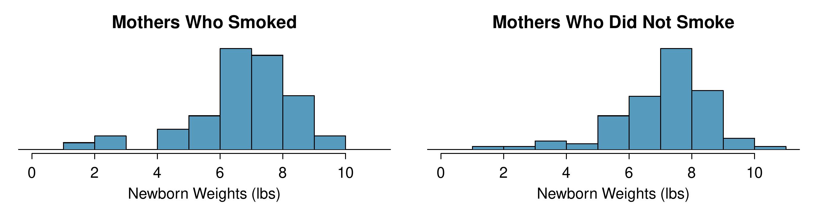
  • With both data sets over 30 observations, we inspect the data in FigureΒ 7.3.7 for any particularly extreme outliers and find none.
Since both conditions are satisfied, the difference in sample means may be modeled using a \(t\)-distribution.
Two histograms are shown for "Newborn Weights, in pounds", one for "Mothers Who Smoked" and one for "Mothers Who Did Not Smoke". The histogram for "Mothers Who Smoked" is centered at about 7 and is left-skewed, with values ranging from about 1 pound to 10 pounds. The histogram for "Mothers Who Did Not Smoke" is centered at about 7.5 and is left-skewed, with values ranging from about 1 pound to 11 pounds.
Figure 7.3.7. The left panel represents birth weights for infants whose mothers smoked. The right panel represents the birth weights for infants whose mothers who did not smoke.

Checkpoint 7.3.8.

The summary statistics in FigureΒ 7.3.9 may be useful for this Guided Practice.
  1. What is the point estimate of the population difference, \(\mu_{n} - \mu_{s}\text{?}\)
  2. Compute the standard error of the point estimate from part (a).
Solution.
(a) The difference in sample means is an appropriate point estimate: \(\bar{x}_{n} - \bar{x}_{s} = 0.40\text{.}\)
(b) The standard error of the estimate can be calculated using the standard error formula:
\begin{align*} SE \amp= \sqrt{\frac{\sigma_n^2}{n_n} + \frac{\sigma_s^2}{n_s}} \approx \sqrt{\frac{s_n^2}{n_n} + \frac{s_s^2}{n_s}}\\ \amp= \sqrt{\frac{1.60^2}{100} + \frac{1.43^2}{50}}\\ \amp= 0.26 \end{align*}
smoker nonsmoker
mean 6.78 7.18
st. dev. 1.43 1.60
samp. size 50 100
Figure 7.3.9. Summary statistics for the ncbirths data set.

Example 7.3.10.

Complete the hypothesis test started in ExampleΒ 7.3.6 and CheckpointΒ 7.3.8. Use a significance level of \(\alpha=0.05\text{.}\) For reference, \(\bar{x}_{n} - \bar{x}_{s} = 0.40\text{,}\) \(SE = 0.26\text{,}\) and the sample sizes were \(n_n = 100\) and \(n_s = 50\text{.}\)
Solution.
We can find the test statistic for this test using the values from CheckpointΒ 7.3.8:
\begin{equation*} T = \frac{0.40 - 0}{0.26} = 1.54 \end{equation*}
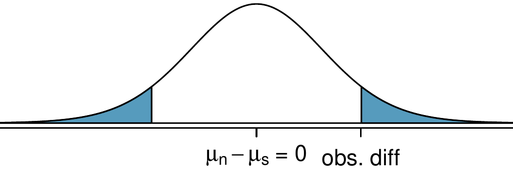
The p-value is represented by the two shaded tails in the following plot:
A bell-shaped curve that resembles a normal distribution is shown centered at "mu-sub-n minus mu-sub-s equals 0". The upper tail is shaded above a value marked as "observed difference", and the corresponding lower tail is also shaded. These tails together appear to represent about 10% to 15% of the area under the distribution.
Figure 7.3.11. Distribution of the difference of sample means for the baby smoke data.
We find the single tail area using software (or the \(t\)-table in the appendix). We’ll use the smaller of \(n_n - 1 = 99\) and \(n_s - 1 = 49\) as the degrees of freedom: \(df = 49\text{.}\) The one tail area is 0.065; doubling this value gives the two-tail area and p-value, 0.135.
The p-value is larger than the significance value, 0.05, so we do not reject the null hypothesis. There is insufficient evidence to say there is a difference in average birth weight of newborns from North Carolina mothers who did smoke during pregnancy and newborns from North Carolina mothers who did not smoke during pregnancy.

Checkpoint 7.3.12.

We’ve seen much research suggesting smoking is harmful during pregnancy, so how could we fail to reject the null hypothesis in ExampleΒ 7.3.10?
Solution.
It is possible that there is a difference but we did not detect it. If there is a difference, we made a Type 2 Error.

Checkpoint 7.3.13.

If we made a Type 2 Error and there is a difference, what could we have done differently in data collection to be more likely to detect the difference?
Solution.
We could have collected more data. If the sample sizes are larger, we tend to have a better shot at finding a difference if one exists. In fact, this is exactly what we would find if we examined a larger data set!
Public service announcement: while we have used this relatively small data set as an example, larger data sets show that women who smoke tend to have smaller newborns. In fact, some in the tobacco industry actually had the audacity to tout that as a benefit of smoking:
It’s true. The babies born from women who smoke are smaller, but they’re just as healthy as the babies born from women who do not smoke. And some women would prefer having smaller babies.
- Joseph Cullman, Philip Morris’ Chairman of the Board on CBS’ Face the Nation, Jan 3, 1971
Fact check: the babies from women who smoke are not actually as healthy as the babies from women who do not smoke.
 1 
You can watch an episode of John Oliver on Last Week Tonight to explore the present day offenses of the tobacco industry. Please be aware that there is some adult language: youtu.be/6UsHHOCH4q8.

Subsection 7.3.3 Case study: two versions of a course exam

An instructor decided to run two slight variations of the same exam. Prior to passing out the exams, she shuffled the exams together to ensure each student received a random version. Summary statistics for how students performed on these two exams are shown in FigureΒ 7.3.14. Anticipating complaints from students who took Version B, she would like to evaluate whether the difference observed in the groups is so large that it provides convincing evidence that Version B was more difficult (on average) than Version A.
Version \(n\) \(\bar{x}\) \(s\) min max
A 30 79.4 14 45 100
B 27 74.1 20 32 100
Figure 7.3.14. Summary statistics of scores for each exam version.

Checkpoint 7.3.15.

Construct hypotheses to evaluate whether the observed difference in sample means, \(\bar{x}_A - \bar{x}_B=5.3\text{,}\) is due to chance. We will later evaluate these hypotheses using \(\alpha = 0.01\text{.}\)
Solution.
\(H_0\text{:}\) the exams are equally difficult, on average. \(\mu_A - \mu_B = 0\text{.}\) \(H_A\text{:}\) one exam was more difficult than the other, on average. \(\mu_A - \mu_B \neq 0\text{.}\)

Checkpoint 7.3.16.

To evaluate the hypotheses in CheckpointΒ 7.3.15 using the \(t\)-distribution, we must first verify conditions.
  1. Does it seem reasonable that the scores are independent?
  2. Any concerns about outliers?
Solution.
(a) Since the exams were shuffled, the β€œtreatment” in this case was randomly assigned, so independence within and between groups is satisfied.
(b) The summary statistics suggest the data are roughly symmetric about the mean, and the min/max values don’t suggest any outliers of concern.
After verifying the conditions for each sample and confirming the samples are independent of each other, we are ready to conduct the test using the \(t\)-distribution. In this case, we are estimating the true difference in average test scores using the sample data, so the point estimate is \(\bar{x}_A - \bar{x}_B = 5.3\text{.}\) The standard error of the estimate can be calculated as
\begin{align*} SE \amp= \sqrt{\frac{s_A^2}{n_A} + \frac{s_B^2}{n_B}}\\ \amp= \sqrt{\frac{14^2}{30} + \frac{20^2}{27}}\\ \amp= 4.62 \end{align*}
Finally, we construct the test statistic:
\begin{align*} T \amp= \frac{\text{point estimate} - \text{null value}}{SE}\\ \amp= \frac{(79.4-74.1) - 0}{4.62}\\ \amp= 1.15 \end{align*}
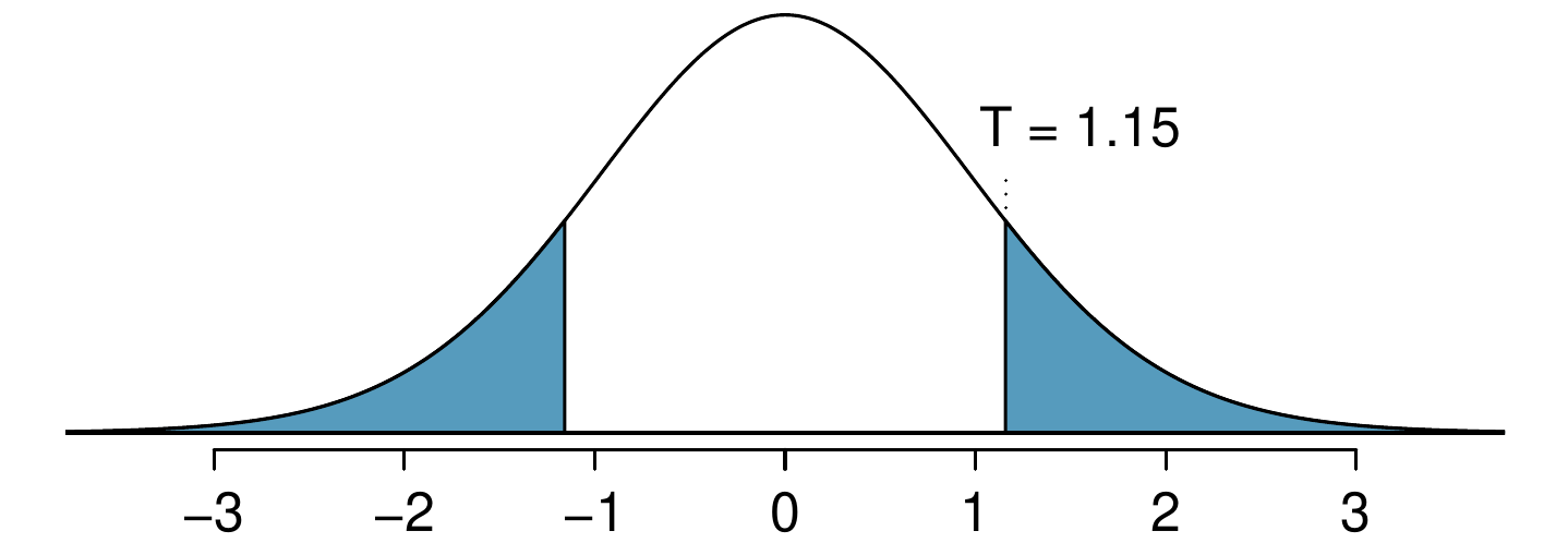
If we have a computer handy, we can identify the degrees of freedom as 45.97. Otherwise we use the smaller of \(n_1-1\) and \(n_2-1\text{:}\) \(df=26\text{.}\)
A t-distribution with 26 degrees of freedom is shown along with the p-value from the exam example represented as shaded area. The t-distribution shown is centered at zero, and the upper tail area above T equals 1.15 is shaded along with the area below about -1.15. These shaded tail areas appear to represent roughly 25% of the distribution.
Figure 7.3.17. The \(t\)-distribution with 26 degrees of freedom and the p-value from exam example represented as the shaded areas.

Example 7.3.18.

Identify the p-value depicted in FigureΒ 7.3.17 using \(df = 26\text{,}\) and provide a conclusion in the context of the case study.
Solution.
Using software, we can find the one-tail area (0.13) and then double this value to get the two-tail area, which is the p-value: 0.26. (Alternatively, we could use the \(t\)-table in the appendix.)
In CheckpointΒ 7.3.15, we specified that we would use \(\alpha = 0.01\text{.}\) Since the p-value is larger than \(\alpha\text{,}\) we do not reject the null hypothesis. That is, the data do not convincingly show that one exam version is more difficult than the other, and the teacher should not be convinced that she should add points to the Version B exam scores.

Subsection 7.3.4 Pooled standard deviation estimate (special topic)

Occasionally, two populations will have standard deviations that are so similar that they can be treated as identical. For example, historical data or a well-understood biological mechanism may justify this strong assumption. In such cases, we can make the \(t\)-distribution approach slightly more precise by using a pooled standard deviation.
The pooled standard deviation of two groups is a way to use data from both samples to better estimate the standard deviation and standard error. If \(s_1\) and \(s_2\) are the standard deviations of groups 1 and 2 and there are very good reasons to believe that the population standard deviations are equal, then we can obtain an improved estimate of the group variances by pooling their data:
\begin{equation*} s_{pooled}^2 = \frac{s_1^2\times (n_1-1) + s_2^2\times (n_2-1)}{n_1 + n_2 - 2} \end{equation*}
where \(n_1\) and \(n_2\) are the sample sizes, as before. To use this new statistic, we substitute \(s_{pooled}^2\) in place of \(s_1^2\) and \(s_2^2\) in the standard error formula, and we use an updated formula for the degrees of freedom:
\begin{equation*} df = n_1 + n_2 - 2 \end{equation*}
The benefits of pooling the standard deviation are realized through obtaining a better estimate of the standard deviation for each group and using a larger degrees of freedom parameter for the \(t\)-distribution. Both of these changes may permit a more accurate model of the sampling distribution of \(\bar{x}_1 - \bar{x}_2\text{,}\) if the standard deviations of the two groups are indeed equal.

Pool standard deviations only after careful consideration.

A pooled standard deviation is only appropriate when background research indicates the population standard deviations are nearly equal. When the sample size is large and the condition may be adequately checked with data, the benefits of pooling the standard deviations greatly diminishes.

Exercises 7.3.5 Exercises

1. Friday the 13\(^{\text{th}}\text{,}\) Part I.

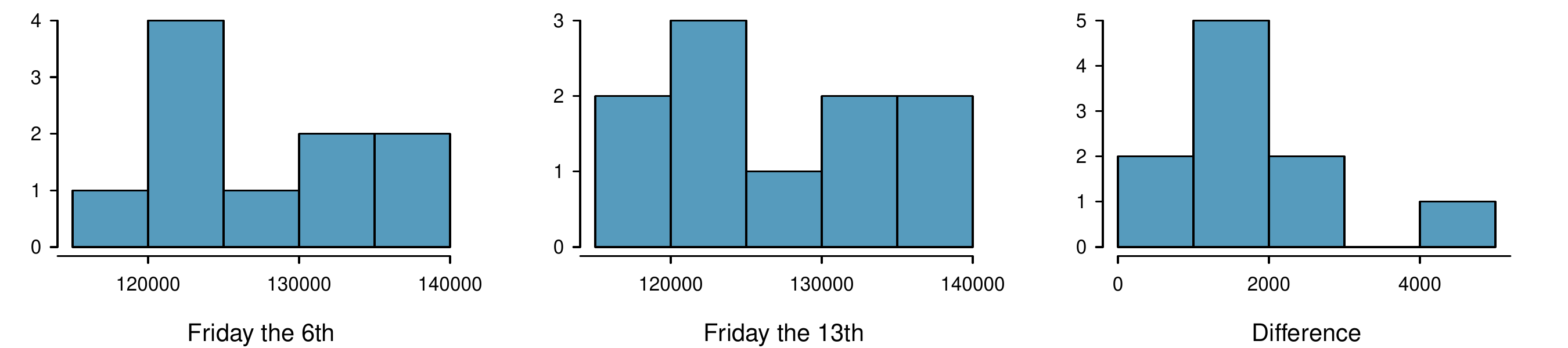
In the early 1990’s, researchers in the UK collected data on traffic flow, number of shoppers, and traffic accident related emergency room admissions on Friday the 13\(^{\text{th}}\) and the previous Friday, Friday the 6\(^{\text{th}}\text{.}\) The histograms below show the distribution of number of cars passing by a specific intersection on Friday the 6\(^{\text{th}}\) and Friday the 13\(^{\text{th}}\) for many such date pairs. Also given are some sample statistics, where the difference is the number of cars on the 6th minus the number of cars on the 13th.
Three histograms are shown. The first histogram is for "Friday the 6th", which has values ranging from 110,000 to 140,000. The second histogram is for "Friday the 13th", which also has values ranging from 110,000 to 140,000. The third histogram is for "Difference", with values ranging from 0 to 5,000. While the first two distributions are relatively uniform across the range, the last distribution has most of its distribution ranging between 0 and 3,000, with one observation in the 4,000 to 5,000 bin.
Figure 7.3.19.
6\(^{\text{th}}\) 13\(^{\text{th}}\) Diff.
\(\bar{x}\) 128,385 126,550 1,835
\(s\) 7,259 7,664 1,176
\(n\) 10 10 10
  1. Are there any underlying structures in these data that should be considered in an analysis? Explain.
  2. What are the hypotheses for evaluating whether the number of people out on Friday the 6\(^{\text{th}}\) is different than the number out on Friday the 13\(^{\text{th}}\text{?}\)
  3. Check conditions to carry out the hypothesis test from part (b).
  4. Calculate the test statistic and the p-value.
  5. What is the conclusion of the hypothesis test?
  6. Interpret the p-value in this context.
  7. What type of error might have been made in the conclusion of your test? Explain.

2. Diamonds, Part I.

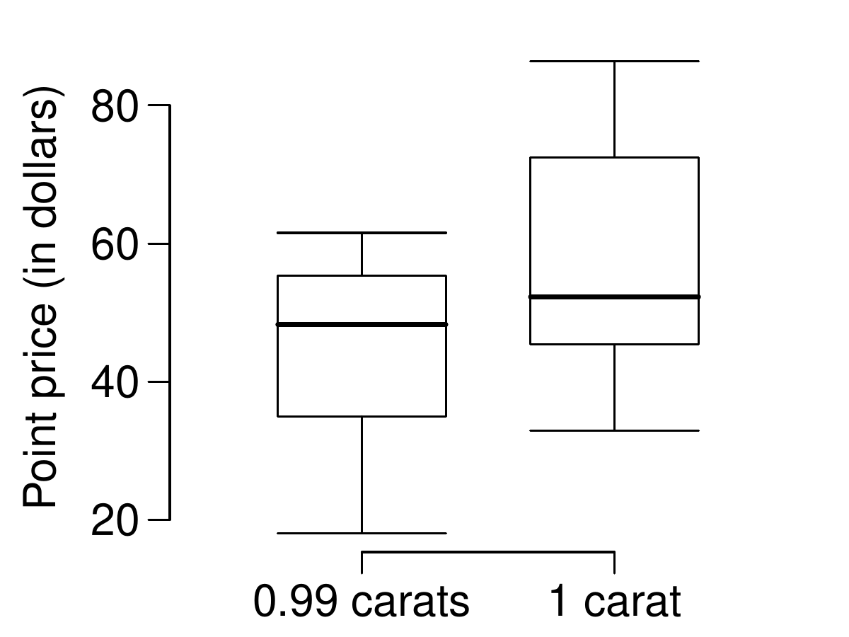
Prices of diamonds are determined by what is known as the 4 Cs: cut, clarity, color, and carat weight. The prices of diamonds go up as the carat weight increases, but the increase is not smooth. For example, the difference between the size of a 0.99 carat diamond and a 1 carat diamond is undetectable to the naked human eye, but the price of a 1 carat diamond tends to be much higher than the price of a 0.99 diamond. In this question we use two random samples of diamonds, 0.99 carats and 1 carat, each sample of size 23, and compare the average prices of the diamonds. In order to be able to compare equivalent units, we first divide the price for each diamond by 100 times its weight in carats. That is, for a 0.99 carat diamond, we divide the price by 99. For a 1 carat diamond, we divide the price by 100. The distributions and some sample statistics are shown below.
Conduct a hypothesis test to evaluate if there is a difference between the average standardized prices of 0.99 and 1 carat diamonds. Make sure to state your hypotheses clearly, check relevant conditions, and interpret your results in context of the data.
0.99 carats 1 carat
Mean $44.51 $56.81
SD $13.32 $16.13
n 23 23
Side-by-side box plot for "Point price, in dollars". The two categories shown are for "0.99 carats" and "1 carat" diamonds. The 0.99 carat diamonds have their box running from about $36 to $57, a median of about $49, and the whiskers spanning about $19 to $62. The 1 carat diamonds have their box running from about $48 to $72, a median of about $55, and the whiskers spanning about $34 to $72.
Figure 7.3.20.

3. Friday the 13\(^{\text{th}}\text{,}\) Part II.

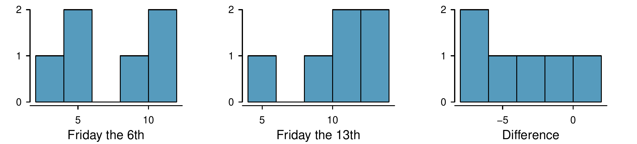
The Friday the \(13^{\text{th}}\) study reported in ExerciseΒ 7.3.5.1 also provides data on traffic accident related emergency room admissions. The distributions of these counts from Friday the 6\(^{\text{th}}\) and Friday the 13\(^{\text{th}}\) are shown below for six such paired dates along with summary statistics. You may assume that conditions for inference are met.
Three histograms are shown. The first histogram is for "Friday the 6th", which has values ranging across 3 to 12. The second histogram is for "Friday the 13th", which has values ranging from 4 to 14. The third histogram is for "Difference", with values ranging from -8 to positive 2.
Figure 7.3.21.
6\(^{\text{th}}\) 13\(^{\text{th}}\) diff
Mean 7.5 10.83 -3.33
SD 3.33 3.6 3.01
n 6 6 6
  1. Conduct a hypothesis test to evaluate if there is a difference between the average numbers of traffic accident related emergency room admissions between Friday the 6\(^{\text{th}}\) and Friday the 13\(^{\text{th}}\text{.}\)
  2. Calculate a 95% confidence interval for the difference between the average numbers of traffic accident related emergency room admissions between Friday the 6\(^{\text{th}}\) and Friday the 13\(^{\text{th}}\text{.}\)
  3. The conclusion of the original study states, "Friday 13th is unlucky for some. The risk of hospital admission as a result of a transport accident may be increased by as much as 52%. Staying at home is recommended." Do you agree with this statement? Explain your reasoning.

4. Diamonds, Part II.

In ExerciseΒ 7.3.5.2, we discussed diamond prices (standardized by weight) for diamonds with weights 0.99 carats and 1 carat. See the table for summary statistics, and then construct a 95% confidence interval for the average difference between the standardized prices of 0.99 and 1 carat diamonds. You may assume the conditions for inference are met.
0.99 carats 1 carat
Mean $44.51 $56.81
SD $13.32 $16.13
n 23 23

5. Chicken diet and weight, Part I.

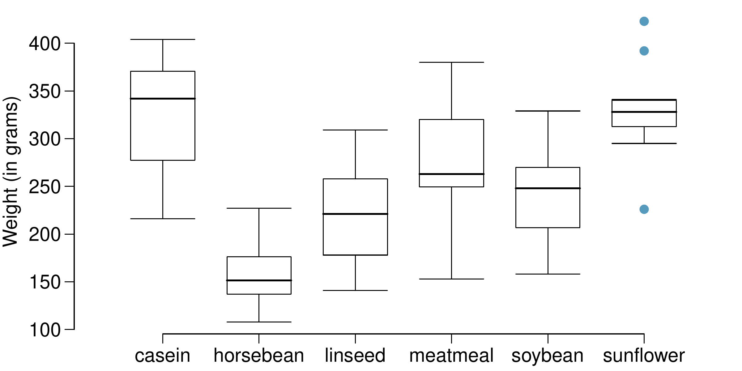
Chicken farming is a multi-billion dollar industry, and any methods that increase the growth rate of young chicks can reduce consumer costs while increasing company profits, possibly by millions of dollars. An experiment was conducted to measure and compare the effectiveness of various feed supplements on the growth rate of chickens. Newly hatched chicks were randomly allocated into six groups, and each group was given a different feed supplement. Below are some summary statistics from this data set along with box plots showing the distribution of weights by feed type.
A side-by-side box plot is shown for "Weight, in grams" for several feed types. The width of the data range for each feed type spans about 150 grams. However, they are centered at different locations: about 325 for "casein", about 150 for "horsebean", about 225 for "linseed", about 275 for "meatmeal", about 250 for "soybean", and about 325 for "sunflower".
Figure 7.3.22.
Mean SD n
casein 323.58 64.43 12
horsebean 160.20 38.63 10
linseed 218.75 52.24 12
meatmeal 276.91 64.90 11
soybean 246.43 54.13 14
sunflower 328.92 48.84 12
  1. Describe the distributions of weights of chickens that were fed linseed and horsebean.
  2. Do these data provide strong evidence that the average weights of chickens that were fed linseed and horsebean are different? Use a 5% significance level.
  3. What type of error might we have committed? Explain.
  4. Would your conclusion change if we used \(\alpha = 0.01\text{?}\)

6. Fuel efficiency of manual and automatic cars, Part I.

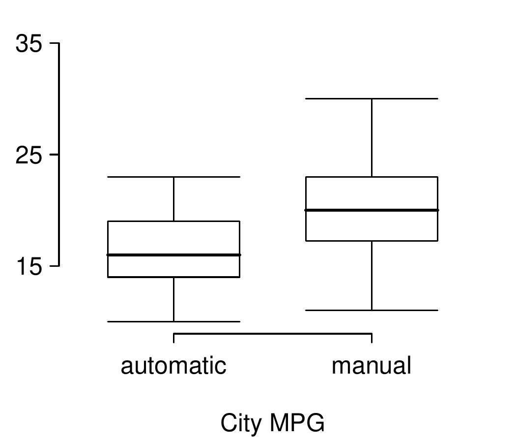
Each year the US Environmental Protection Agency (EPA) releases fuel economy data on cars manufactured in that year. Below are summary statistics on fuel efficiency (in miles/gallon) from random samples of cars with manual and automatic transmissions. Do these data provide strong evidence of a difference between the average fuel efficiency of cars with manual and automatic transmissions in terms of their average city mileage? Assume that conditions for inference are satisfied.
City MPG
Automatic Manual
Mean 16.12 19.85
SD 3.58 4.51
n 26 26
A side-by-side box plot is shown for "City MPG" for "automatic" and "manual" cars. The "automatic" box plot has its box spanning approximately 14 to 19, has a median of about 16, and its whiskers extending down to about 7 and up to about 24. The "manual" box plot has its box spanning approximately 18 to 24, has a median of about 21, and its whiskers extending down to about 8 and up to about 31.
Figure 7.3.23.

7. Chicken diet and weight, Part II.

Casein is a common weight gain supplement for humans. Does it have an effect on chickens? Using data provided in ExerciseΒ 7.3.5.5, test the hypothesis that the average weight of chickens that were fed casein is different than the average weight of chickens that were fed soybean. If your hypothesis test yields a statistically significant result, discuss whether or not the higher average weight of chickens can be attributed to the casein diet. Assume that conditions for inference are satisfied.

8. Fuel efficiency of manual and automatic cars, Part II.

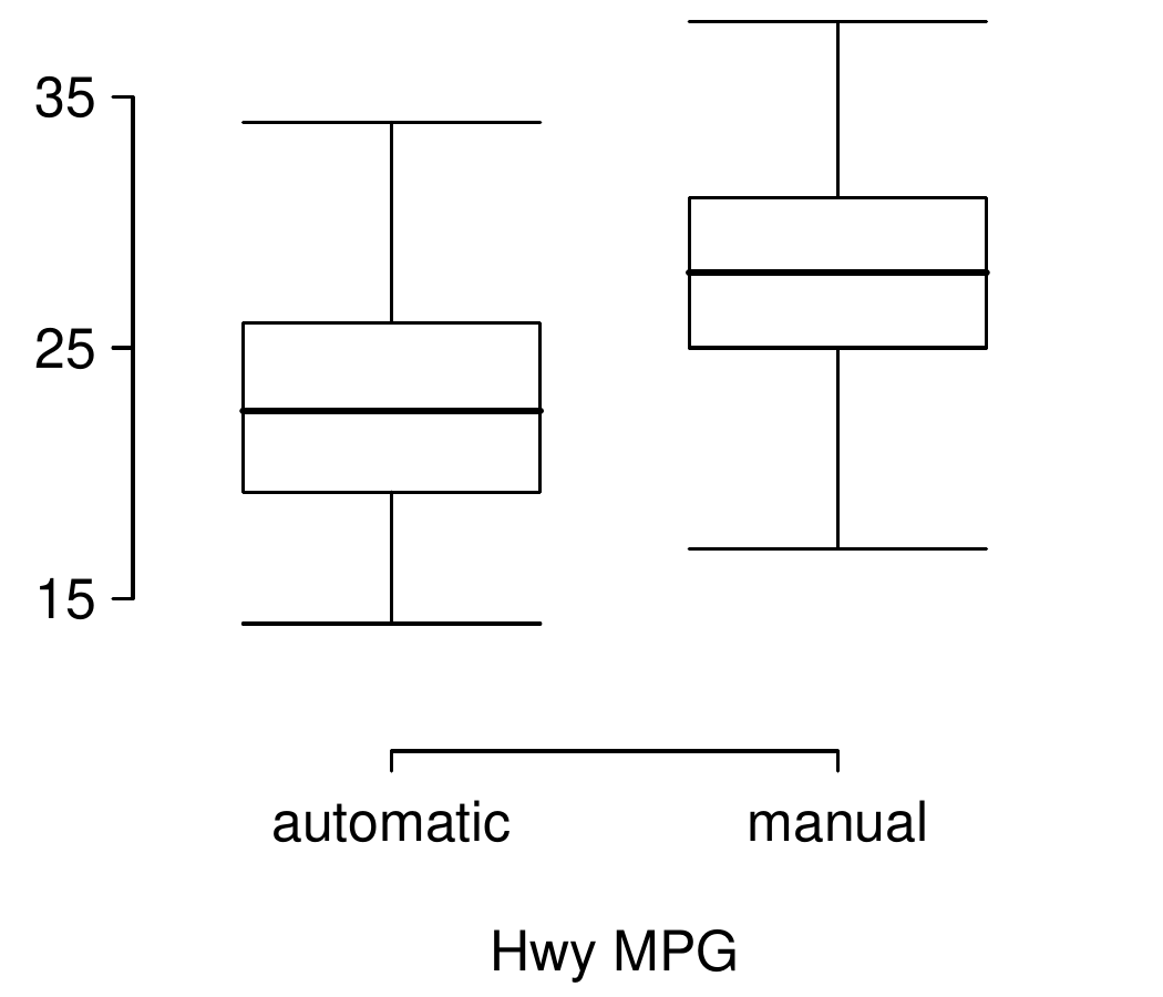
The table provides summary statistics on highway fuel economy of the same 52 cars from ExerciseΒ 7.3.5.6. Use these statistics to calculate a 98% confidence interval for the difference between average highway mileage of manual and automatic cars, and interpret this interval in the context of the data.
Hwy MPG
Automatic Manual
Mean 22.92 27.88
SD 5.29 5.01
n 26 26
A side-by-side box plot is shown for "Highway MPG" for "automatic" and "manual" cars. The "automatic" box plot has its box spanning approximately 20 to 26, has a median of about 23, and its whiskers extending down to about 14 and up to about 34. The "manual" box plot has its box spanning approximately 26 to 32, has a median of about 29, and its whiskers extending down to about 17 and up to about 38.
Figure 7.3.24.

9. Prison isolation experiment, Part I.

Subjects from Central Prison in Raleigh, NC, volunteered for an experiment involving an "isolation" experience. The goal of the experiment was to find a treatment that reduces subjects’ psychopathic deviant T scores. This score measures a person’s need for control or their rebellion against control, and it is part of a commonly used mental health test called the Minnesota Multiphasic Personality Inventory (MMPI) test. The experiment had three treatment groups:
  1. Four hours of sensory restriction plus a 15 minute "therapeutic" tape advising that professional help is available.
  2. Four hours of sensory restriction plus a 15 minute "emotionally neutral" tape on training hunting dogs.
  3. Four hours of sensory restriction but no taped message.
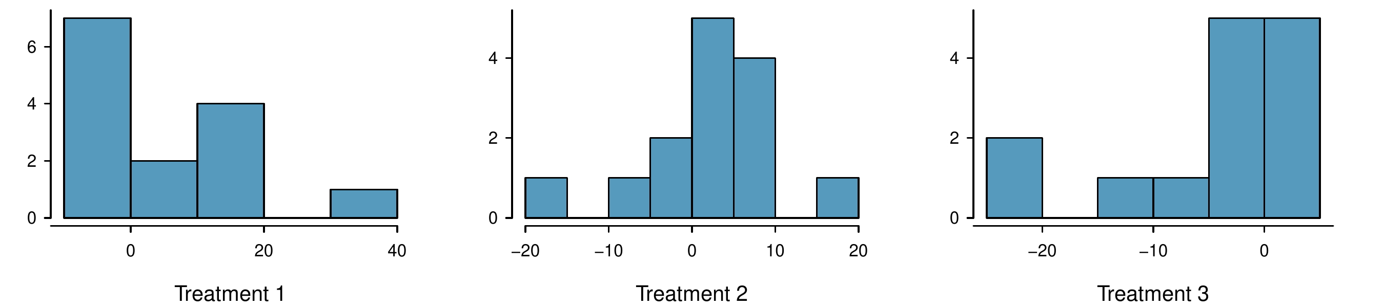
Forty-two subjects were randomly assigned to these treatment groups, and an MMPI test was administered before and after the treatment. Distributions of the differences between pre and post treatment scores (pre - post) are shown below, along with some sample statistics. Use this information to independently test the effectiveness of each treatment. Make sure to clearly state your hypotheses, check conditions, and interpret results in the context of the data.
Three box plots are shown for Treatments 1, 2, and 3. The box plot for "Treatment 1" is slightly right skewed with values ranging from about -10 to about positive 40, and this distribution has one borderline outlier between 30 and 40. The box plot for "Treatment 2" is about symmetric with values ranging from about -20 to about positive 20. The box plot for "Treatment 3" is left skewed with values ranging from about -30 to about positive 10.
Figure 7.3.25.
Tr 1 Tr 2 Tr 3
Mean 6.21 2.86 -3.21
SD 12.3 7.94 8.57
n 14 14 14

10. True / False: comparing means.

Determine if the following statements are true or false, and explain your reasoning for statements you identify as false.
  1. When comparing means of two samples where \(n_1 = 20\) and \(n_2 = 40\text{,}\) we can use the normal model for the difference in means since \(n_2 \ge 30\text{.}\)
  2. As the degrees of freedom increases, the \(t\)-distribution approaches normality.
  3. We use a pooled standard error for calculating the standard error of the difference between means when sample sizes of groups are equal to each other.