Introductory Statistics

Section 9.4 Multiple regression case study: Mario Kart

Weโ€™ll consider eBay auctions of a video game called Mario Kart for the Nintendo Wii. The outcome variable of interest is the total price of an auction, which is the highest bid plus the shipping cost. We will try to determine how total price is related to each characteristic in an auction while simultaneously controlling for other variables. For instance, all other characteristics held constant, are longer auctions associated with higher or lower prices? And, on average, how much more do buyers tend to pay for additional Wii wheels (plastic steering wheels that attach to the Wii controller) in auctions? Multiple regression will help us answer these and other questions.

Subsection 9.4.1 Data set and the full model

The mariokart data set includes results from 141 auctions. Four observations from this data set are shown in Figureย 9.4.1, and descriptions for each variable are shown in Figureย 9.4.2. Notice that the condition and stock photo variables are indicator variables, similar to bankruptcy in the loans data set.
price cond_new stock_photo duration wheels
1 51.55 1 1 3 1
2 37.04 0 1 7 1
\(\vdots\) \(\vdots\) \(\vdots\) \(\vdots\) \(\vdots\) \(\vdots\)
140 38.76 0 0 7 0
141 54.51 1 1 1 2
Figure 9.4.1. Four observations from the mariokart data set.
variable description
price Final auction price plus shipping costs, in US dollars.
cond_new Indicator variable for if the game is new (1) or used (0).
stock_photo Indicator variable for if the auctionโ€™s main photo is a stock photo.
duration The length of the auction, in days, taking values from 1 to 10.
wheels The number of Wii wheels included with the auction. A Wii wheel is an optional steering wheel accessory that holds the Wii controller.
Figure 9.4.2. Variables and their descriptions for the mariokart data set.

Checkpoint 9.4.3.

We fit a linear regression model with the gameโ€™s condition as a predictor of auction price. Results of this model are summarized below:
Estimate Std. Error t value Pr(\(>\)|t|)
(Intercept) 42.8711 0.8140 52.67 \(\lt\)0.0001
cond_new 10.8996 1.2583 8.66 \(\lt\)0.0001
\(df=139\)
Write down the equation for the model, note whether the slope is statistically different from zero, and interpret the coefficient.
Solution.
The equation for the line may be written as
\begin{equation*} \widehat{\text{price}} = 42.87 + 10.90 \times \text{cond\_new} \end{equation*}
Examining the regression output, we can see that the p-value for cond_new is very close to zero, indicating there is strong evidence that the coefficient is different from zero when using this simple one-variable model.
The cond_new is a two-level categorical variable that takes value 1 when the game is new and value 0 when the game is used. This means the 10.90 model coefficient predicts an extra $10.90 for those games that are new versus those that are used.
Sometimes there are underlying structures or relationships between predictor variables. For instance, new games sold on eBay tend to come with more Wii wheels, which may have led to higher prices for those auctions. We would like to fit a model that includes all potentially important variables simultaneously. This would help us evaluate the relationship between a predictor variable and the outcome while controlling for the potential influence of other variables.
We want to construct a model that accounts for not only the game condition, as in Checkpointย 9.4.3, but simultaneously accounts for three other variables:
\begin{align*} \widehat{\text{price}} \amp = \beta_0 + \beta_1 \times \text{cond\_new} + \beta_2 \times \text{stock\_photo}\\ \amp \qquad + \beta_3 \times \text{duration} + \beta_4 \times \text{wheels} \end{align*}
Figureย 9.4.4 summarizes the full model. Using this output, we identify the point estimates of each coefficient.
Estimate Std. Error t value Pr(\(>\)|t|)
(Intercept) 36.2110 1.5140 23.92 \(\lt\)0.0001
cond_new 5.1306 1.0511 4.88 \(\lt\)0.0001
stock_photo 1.0803 1.0568 1.02 0.3085
duration -0.0268 0.1904 -0.14 0.8882
wheels 7.2852 0.5547 13.13 \(\lt\)0.0001
\(df=136\)
Figure 9.4.4. Output for the regression model where price is the outcome and cond_new, stock_photo, duration, and wheels are the predictors.

Checkpoint 9.4.5.

Write out the modelโ€™s equation using the point estimates from Figureย 9.4.4. How many predictors are there in this model?
Solution.
\begin{align*} \widehat{\text{price}} \amp = 36.21 + 5.13 \times \text{cond\_new} + 1.08 \times \text{stock\_photo}\\ \amp \qquad - 0.03 \times \text{duration} + 7.29 \times \text{wheels} \end{align*}
with the \(k=4\) predictors.

Checkpoint 9.4.6.

What does \(\beta_4\text{,}\) the coefficient of variable \(x_4\) (Wii wheels), represent? What is the point estimate of \(\beta_4\text{?}\)
Solution.
It is the average difference in auction price for each additional Wii wheel included when holding the other variables constant. The point estimate is \(b_4 = 7.29\text{.}\)

Checkpoint 9.4.7.

Example 9.4.8. Why does the condition coefficient differ between models?

We estimated a coefficient for cond_new in Checkpointย 9.4.3 of \(b_1 = 10.90\) with a standard error of \(SE_{b_1} = 1.26\) when using simple linear regression. Why might there be a difference between that estimate and the one in the multiple regression setting?
Solution.
If we examined the data carefully, we would see that there is collinearity among some predictors. For instance, when we estimated the connection of the outcome price and predictor cond_new using simple linear regression, we were unable to control for other variables like the number of Wii wheels included in the auction. That model was biased by the confounding variable wheels. When we use both variables, this particular underlying and unintentional bias is reduced or eliminated (though bias from other confounding variables may still remain).

Subsection 9.4.2 Model selection

Letโ€™s revisit the model for the Mario Kart auction and complete model selection using backward selection. Recall that the full model took the following form:
\begin{equation*} \widehat{\text{price}} = 36.21 + 5.13 \times \text{cond\_new} + 1.08 \times \text{stock\_photo} - 0.03 \times \text{duration} + 7.29 \times \text{wheels} \end{equation*}

Example 9.4.9. Backward elimination with Mario Kart data.

Results corresponding to the full model for the mariokart data were shown in Figureย 9.4.4. For this model, we consider what would happen if dropping each of the variables in the model:
Exclude... cond_new stock_photo duration wheels
\(R^2_{adj} = 0.6626\) \(R^2_{adj} = 0.7107\) \(R^2_{adj} = 0.7128\) \(R^2_{adj} = 0.3487\)
For the full model, \(R_{adj}^2 = 0.7108\text{.}\) How should we proceed under the backward elimination strategy?
Solution.
The third model without duration has the highest \(R_{adj}^2\) of 0.7128, so we compare it to \(R_{adj}^2\) for the full model. Because eliminating duration leads to a model with a higher \(R_{adj}^2\text{,}\) we drop duration from the model.

Checkpoint 9.4.10.

In Exampleย 9.4.9, we eliminated the duration variable, which resulted in a model with \(R_{adj}^2 = 0.7128\text{.}\) Letโ€™s look at if we would eliminate another variable from the model using backward elimination:
Exclude duration and... cond_new stock_photo wheels
\(R^2_{adj} = 0.6587\) \(R^2_{adj} = 0.7124\) \(R^2_{adj} = 0.3414\)
Should we eliminate any additional variable, and if so, which variable should we eliminate?
Solution.
Removing any of the three remaining variables would lead to a decrease in \(R_{adj}^2\text{,}\) so we should not remove any additional variables from the model after we removed duration.

Checkpoint 9.4.11.

After eliminating the auctionโ€™s duration from the model, we are left with the following reduced model:
\begin{equation*} \widehat{\text{price}} = 36.05 + 5.18 \times \text{cond\_new} + 1.12 \times \text{stock\_photo} + 7.30 \times \text{wheels} \end{equation*}
How much would you predict for the total price for the Mario Kart game if it was used, used a stock photo, and included two wheels and put up for auction during the time period that the Mario Kart data were collected?
Solution.
We would plug in 0 for cond_new, 1 for stock_photo, and 2 for wheels into the equation, which would return $51.77, which is the total price we would expect for the auction.

Checkpoint 9.4.12.

Would you be surprised if the seller from Checkpointย 9.4.11 didnโ€™t get the exact price predicted?
Solution.
No. The model provides the average auction price we would expect, and the price for one auction to the next will continue to vary a bit (but less than what our prediction would be without the model).

Subsection 9.4.3 Checking model conditions using graphs

Letโ€™s take a closer look at the diagnostics for the Mario Kart model to check if the model we have identified is reasonable.
Check for outliers
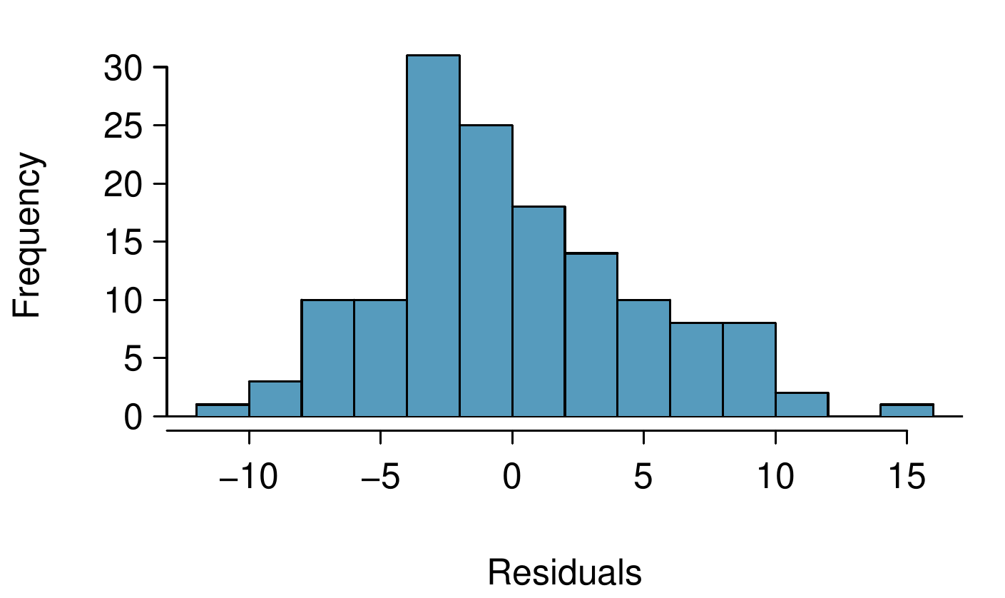
A histogram of the residuals is shown in Figureย 9.4.13. With a data set well over a hundred, weโ€™re primarily looking for major outliers. While one minor outlier appears on the upper end, it is not a concern for this large of a data set.
A histogram is shown for "Residuals". The distribution is centered at 0, is slightly right skewed, and has a standard deviation of about 4.
Figure 9.4.13. Histogram of the residuals. No clear outliers are evident.
Absolute values of residuals against fitted values
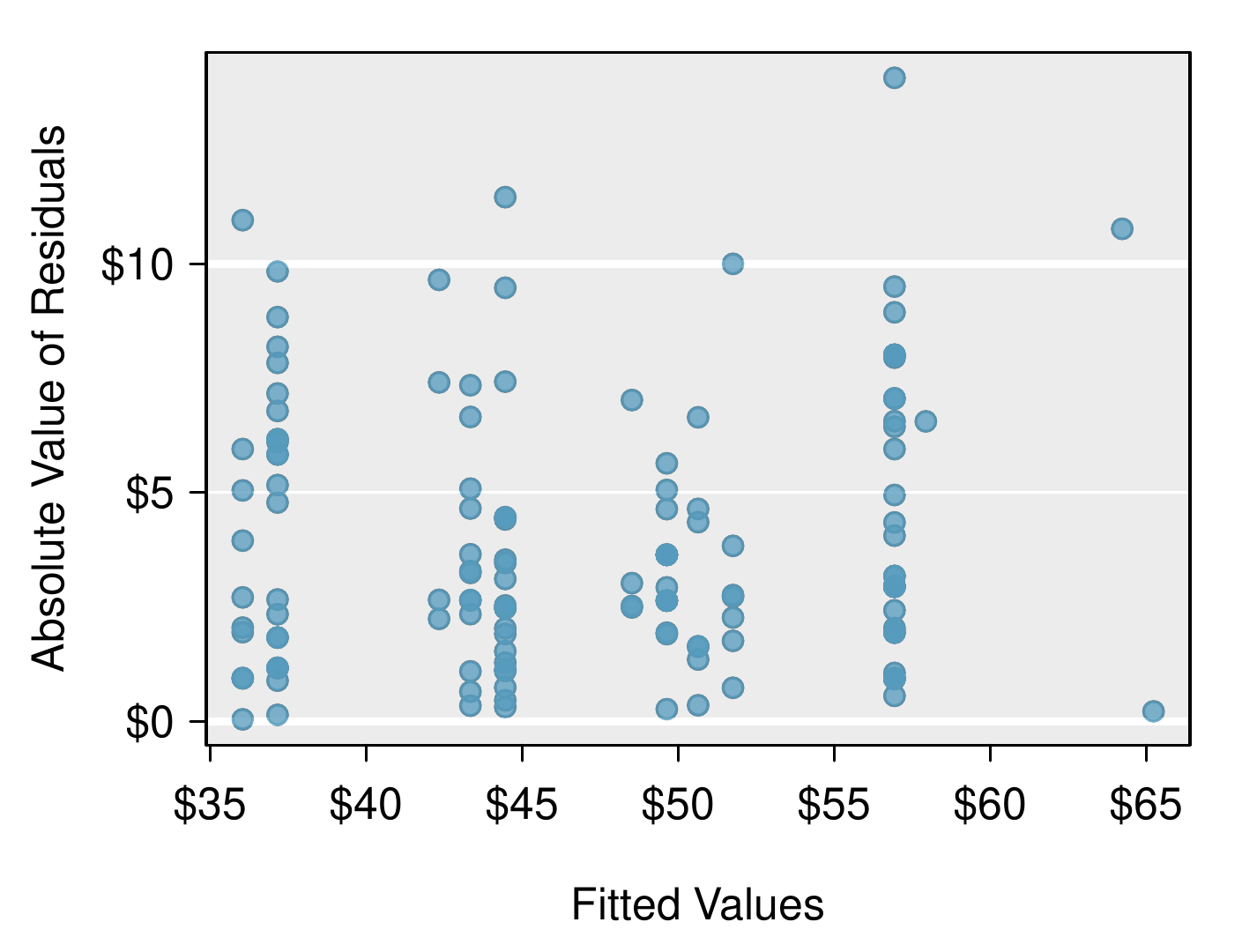
A plot of the absolute value of the residuals against their corresponding fitted values (\(\hat{y}_i\)) is shown in Figureย 9.4.14. We donโ€™t see any obvious deviations from constant variance in this example.
Scatterplot of "Absolute Value of Residuals" (vertical axis) against "Fitted Values" (horizontal axis). The fitted values range from $35 to $65, and the absolute value of the residuals range from $0 to about $10, with no apparent pattern across the range of fitted values.
Figure 9.4.14. Absolute value of the residuals against the fitted values. No patterns are evident.
Residuals in order of their data collection
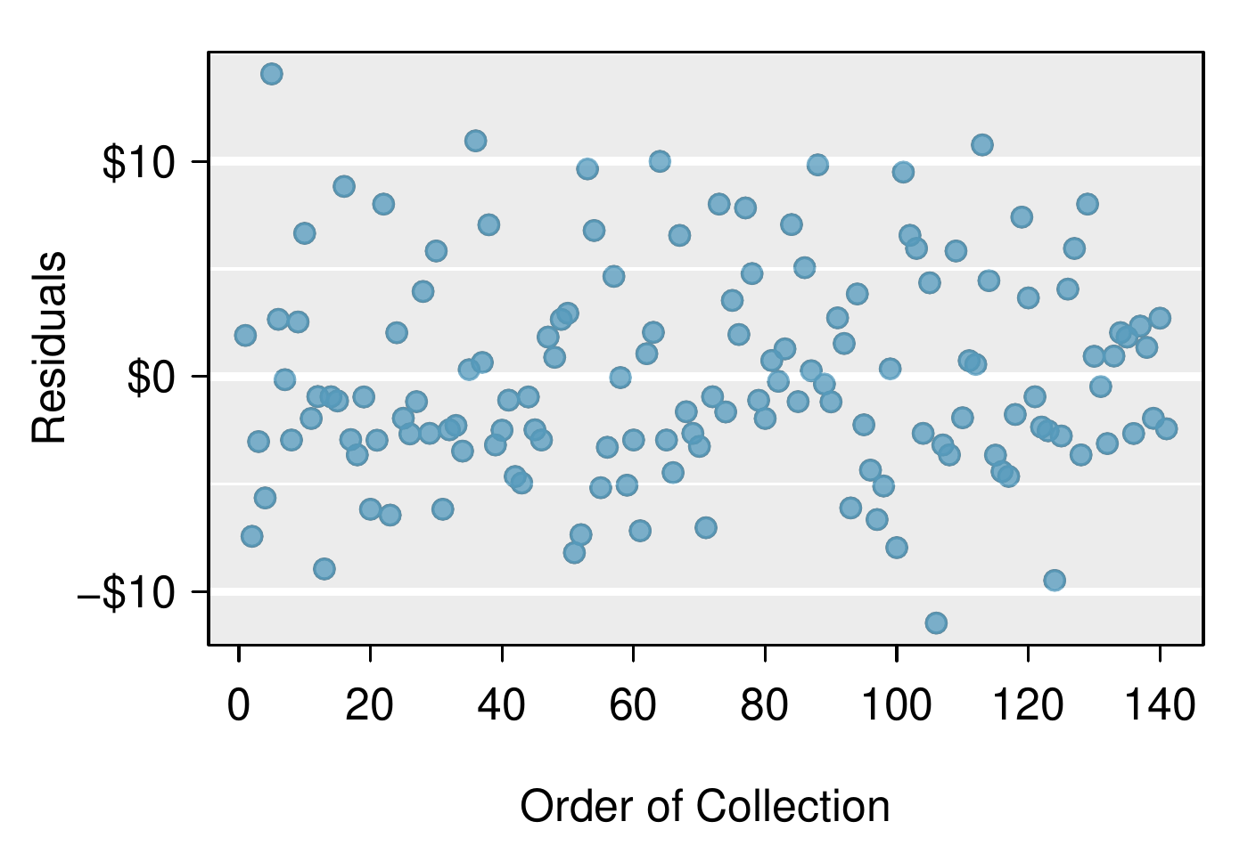
A plot of the residuals in the order their corresponding auctions were observed is shown in Figureย 9.4.15. Here we see no structure that indicates a problem.
Scatterplot of "Residuals" (vertical axis) against "Order of Collection" (horizontal axis). The order of collection runs from 1 to about 140, and the residuals range from -$10 to about positive $10, with no apparent pattern across the range of fitted values.
Figure 9.4.15. Residuals in the order that their corresponding observations were collected. There are no evident patterns.
Residuals against each predictor variable
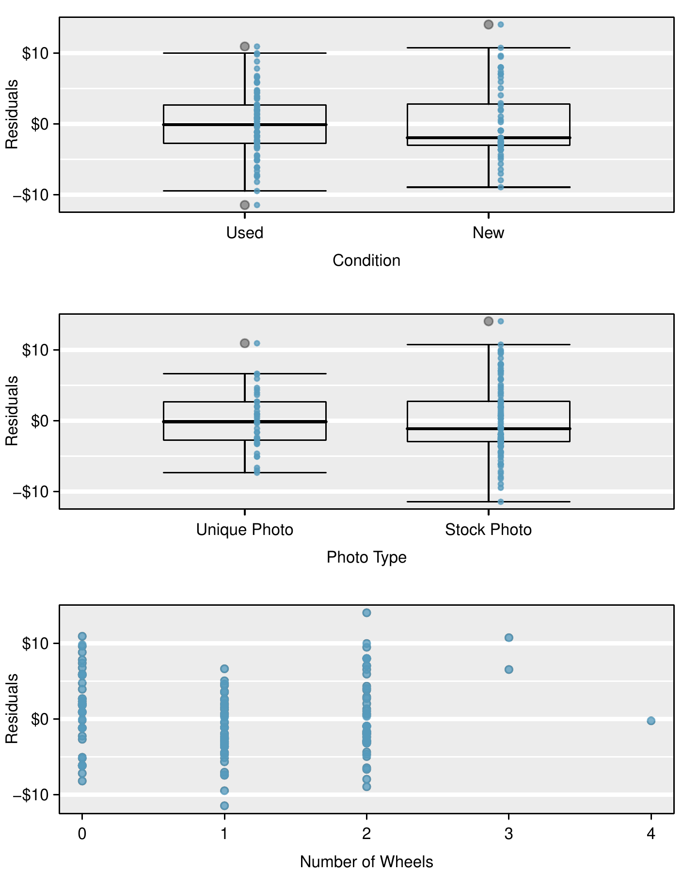
We consider a plot of the residuals against the cond_new variable, the residuals against the stock_photo variable, and the residuals against the wheels variable. These plots are shown in Figureย 9.4.16. For the two-level condition variable, we are guaranteed not to see any remaining trend, and instead we are checking that the variability doesnโ€™t fluctuate across groups, which it does not. However, looking at the stock photo variable, we find that there is some difference in the variability of the residuals in the two groups. Additionally, when we consider the residuals against the wheels variable, we see some possible structure. There appears to be curvature in the residuals, indicating the relationship is probably not linear.
Three plots are shown for "Residuals" against different predictor variables "Condition", "Photo Type", and "Number of Wheels". Condition plot: A side-by-side box plot is shown for the condition levels of "Used" and "New". The median of "Used" is at $0 while the median of "New" is at about -$2. The boxes in each box plot ranges from about -$3 to positive $3, and the whiskers of each box plot runs from about -$10 to positive $10. There are a couple of points slightly beyond the whiskers. Photo Type plot: A side-by-side box plot is shown for the photo type levels of "Unique Photo" and "Stock Photo". The median of "Unique Photos" is at $0 while the median of "Stock Photo" is at about -$1. The boxes in each box plot ranges from about -$3 to positive $3. The whiskers of "Unique Photo" box plot ranges from about -$8 to positive $7, and the whiskers of "Stock Photo" box plot ranges from about -$11 to positive $11. There are a couple of points slightly beyond the whiskers. Number of Wheels plot: A scatterplot is shown for "Residuals" (vertical axis) against "Number of Wheels" (horizontal axis) with values from 0 to 4. For 0 wheels, the residuals largely range from -$8 to positive $10. For 1 wheel, the residuals largely range from -$10 to positive $5. For 2 wheels, the residuals largely range from -$8 to positive $10. There are two points with 3 wheels that have residuals of $6 and $11, and one point with 4 wheels that has a residual of about $0.
Figure 9.4.16. For the condition and stock photo variables, we check for differences in the distribution shape or variability of the residuals. In the case of the stock photos variable, we see a little less variability in the unique photo group than the stock photo group. For numerical predictors, we also check for trends or other structure. We see some slight bowing in the residuals against the wheels variable in the bottom plot.
As with the loans analysis, we would summarize diagnostics when reporting the model results. In the case of this auction data, we would report that there appears to be non-constant variance in the stock photo variable and that there may be a nonlinear relationship between the total price and the number of wheels included for an auction. This information would be important to buyers and sellers who may review the analysis, and omitting this information could be a setback to the very people who the model might assist.
Note: there are no exercises for this section.