Section6.4Testing for independence in two-way tables
We all buy used products — cars, computers, textbooks, and so on — and we sometimes assume the sellers of those products will be forthright about any underlying problems with what they’re selling. This is not something we should take for granted. Researchers recruited 219 participants in a study where they would sell a used iPod 1
For readers not as old as the authors, an iPod is basically an iPhone without any cellular service, assuming it was one of the later generations. Earlier generations were more basic.
that was known to have frozen twice in the past. The participants were incentivized to get as much money as they could for the iPod since they would receive a 5% cut of the sale on top of $10 for participating. The researchers wanted to understand what types of questions would elicit the seller to disclose the freezing issue.
Unbeknownst to the participants who were the sellers in the study, the buyers were collaborating with the researchers to evaluate the influence of different questions on the likelihood of getting the sellers to disclose the past issues with the iPod. The scripted buyers started with “Okay, I guess I’m supposed to go first. So you’ve had the iPod for 2 years …” and ended with one of three questions:
The question is the treatment given to the sellers, and the response is whether the question prompted them to disclose the freezing issue with the iPod. The results are shown in Table 6.4.1, and the data suggest that asking What problems does it have? was the most effective at getting the seller to disclose the past freezing issues. However, you should also be asking yourself: could we see these results due to chance alone, or is this in fact evidence that some questions are more effective for getting at the truth?
A one-way table describes counts for each outcome in a single variable. A two-way table describes counts for combinations of outcomes for two variables. When we consider a two-way table, we often would like to know, are these variables related in any way? That is, are they dependent (versus independent)?
The hypothesis test for the iPod experiment is really about assessing whether there is statistically significant evidence of the success each question had on getting the participant to disclose the problem with the iPod. In other words, the goal is to check whether the buyer’s question was independent of whether the seller disclosed a problem.
Example6.4.2.Computing expected counts for the General group.
From the experiment, we can compute the proportion of all sellers who disclosed the freezing problem as \(61/219 = 0.2785\text{.}\) If there really is no difference among the questions and 27.85% of sellers were going to disclose the freezing problem no matter the question that was put to them, how many of the 73 people in the General group would we have expected to disclose the freezing problem?
We would predict that \(0.2785 \times 73 = 20.33\) sellers would disclose the problem. Obviously we observed fewer than this, though it is not yet clear if that is due to chance variation or whether that is because the questions vary in how effective they are at getting to the truth.
If the questions were actually equally effective, meaning about 27.85% of respondents would disclose the freezing issue regardless of what question they were asked, about how many sellers would we expect to hide the freezing problem from the Positive Assumption group?
We can compute the expected number of sellers who we would expect to disclose or hide the freezing issue for all groups, if the questions had no impact on what they disclosed, using the same strategy employed in Example 6.4.2 and Checkpoint 6.4.3. These expected counts were used to construct Table 6.4.4, which is the same as Table 6.4.1, except now the expected counts have been added in parentheses.
The examples and exercises above provided some help in computing expected counts. In general, expected counts for a two-way table may be computed using the row totals, column totals, and the table total. For instance, if there was no difference between the groups, then about 27.85% of each column should be in the first row:
Looking back to how 0.2785 was computed — as the fraction of sellers who disclosed the freezing issue (\(61/219\)) — these three expected counts could have been computed as
This leads us to a general formula for computing expected counts in a two-way table when we would like to test whether there is strong evidence of an association between the column variable and row variable.
Just like before, this test statistic follows a chi-square distribution. However, the degrees of freedom are computed a little differently for a two-way table. 2
Recall: in the one-way table, the degrees of freedom was the number of cells minus 1.
For two-way tables, the degrees of freedom is equal to
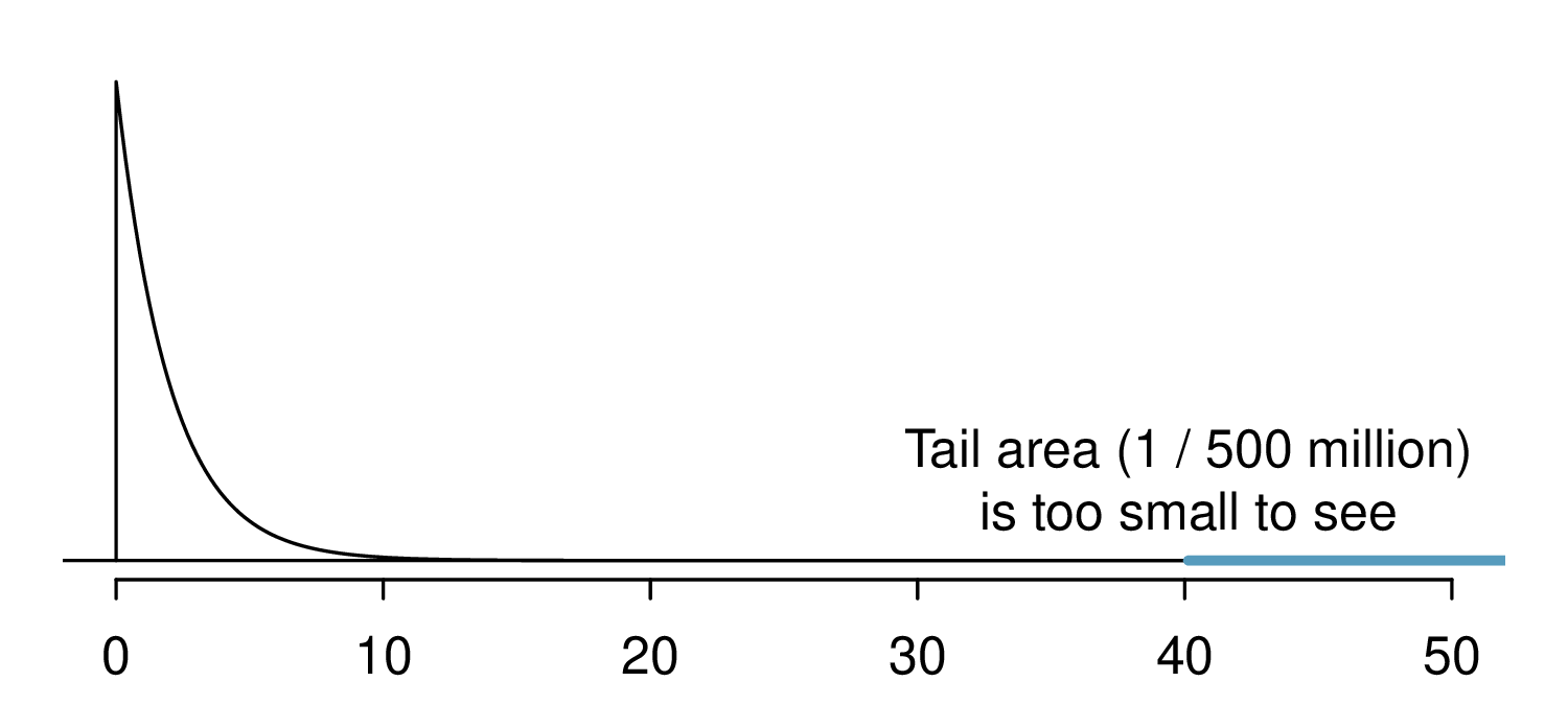
If the null hypothesis is true (i.e. the questions had no impact on the sellers in the experiment), then the test statistic \(X^2 = 40.13\) closely follows a chi-square distribution with 2 degrees of freedom. Using this information, we can compute the p-value for the test, which is depicted in Figure 6.4.5.
Using a computer, we can compute a very precise value for the tail area above \(X^2 = 40.13\) for a chi-square distribution with 2 degrees of freedom: 0.000000002. (If using the table in Appendix C, we would identify the p-value is smaller than 0.001.) Using a significance level of \(\alpha=0.05\text{,}\) the null hypothesis is rejected since the p-value is smaller. That is, the data provide convincing evidence that the question asked did affect a seller’s likelihood to tell the truth about problems with the iPod.
Table 6.4.8 summarizes the results of an experiment evaluating three treatments for Type 2 Diabetes in patients aged 10-17 who were being treated with metformin. The three treatments considered were continued treatment with metformin (met), treatment with metformin combined with rosiglitazone (rosi), or a lifestyle intervention program. Each patient had a primary outcome, which either lacked glycemic control (failure) or did not lack that control (success). What are appropriate hypotheses for this test?
\(H_A\text{:}\) There is some difference in effectiveness between the three treatments, e.g. perhaps the rosi treatment performed better than lifestyle.
A chi-square test for a two-way table may be used to test the hypotheses in Example 6.4.7. As a first step, compute the expected values for each of the six table cells.
The expected count for row one / column one is found by multiplying the row one total (234) and column one total (319), then dividing by the table total (699): \(\frac{234\times 319}{699} = 106.8\text{.}\) Similarly for the second column and the first row: \(\frac{234\times 380}{699} = 127.2\text{.}\) Row 2: 105.9 and 126.1. Row 3: 106.3 and 126.7.
For each cell, compute \(\frac{(\text{obs} - \text{exp})^2}{\text{exp}}\text{.}\) For instance, the first row and first column: \(\frac{(109-106.8)^2}{106.8} = 0.05\text{.}\) Adding the results of each cell gives the chi-square test statistic: \(X^2 = 0.05 + \cdots + 2.11 = 8.16\text{.}\)
Because there are 3 rows and 2 columns, the degrees of freedom for the test is \(df = (3 - 1) \times (2 - 1) = 2\text{.}\) Use \(X^2 = 8.16\text{,}\)\(df = 2\text{,}\) and evaluate whether to reject the null hypothesis using a significance level of 0.05.
If using a computer, we can identify the p-value as 0.017. That is, we reject the null hypothesis because the p-value is less than 0.05, and we conclude that at least one of the treatments is more or less effective than the others at treating Type 2 Diabetes for glycemic control.
Does being part of a support group affect the ability of people to quit smoking? A county health department enrolled 300 smokers in a randomized experiment. 150 participants were assigned to a group that used a nicotine patch and met weekly with a support group; the other 150 received the patch and did not meet with a support group. At the end of the study, 40 of the participants in the patch plus support group had quit smoking while only 30 smokers had quit in the other group.
Answer each of the following questions under the null hypothesis that being part of a support group does not affect the ability of people to quit smoking, and indicate whether the expected values are higher or lower than the observed values.
The table below summarizes a data set we first encountered in an earlier exercise regarding views on full-body scans and political affiliation. The differences in each political group may be due to chance. Complete the following computations under the null hypothesis of independence between an individual’s party affiliation and their support of full-body scans. It may be useful to first add on an extra column for row totals before proceeding with the computations.
The table below summarizes a data set we first encountered in an earlier exercise that examines the responses of a random sample of college graduates and non-graduates on the topic of oil drilling. Complete a chi-square test for these data to check whether there is a statistically significant difference in responses from college graduates and non-graduates.
Lymphatic filariasis is a disease caused by a parasitic worm. Complications of the disease can lead to extreme swelling and other complications. Here we consider results from a randomized experiment that compared three different drug treatment options to clear people of this parasite, which people are working to eliminate entirely. The results for the second year of the study are given below: