Confidence Intervals for a Proportion

Section 5.2 Confidence Intervals for a Proportion

The sample proportion \(\hat{p}\) provides a single plausible value for the population proportion \(p\text{.}\) However, the sample proportion isn’t perfect and will have some standard error associated with it. When stating an estimate for the population proportion, it is better practice to provide a plausible range of values instead of supplying just the point estimate.

🔗

Subsection 5.2.1 Capturing the Population Parameter

Using only a point estimate is like fishing in a murky lake with a spear. We can throw a spear where we saw a fish, but we will probably miss. On the other hand, if we toss a net in that area, we have a good chance of catching the fish. A confidence interval is like fishing with a net, and it represents a range of plausible values where we are likely to find the population parameter.

🔗

If we report a point estimate \(\hat{p}\text{,}\) we probably will not hit the exact population proportion. On the other hand, if we report a range of plausible values, representing a confidence interval, we have a good shot at capturing the parameter.

🔗

Checkpoint 5.2.1.

If we want to be very certain we capture the population proportion in an interval, should we use a wider interval or a smaller interval?

🔗

Solution.

If we want to be more certain we will capture the fish, we might use a wider net. Likewise, we use a wider confidence interval if we want to be more certain that we capture the parameter.

🔗

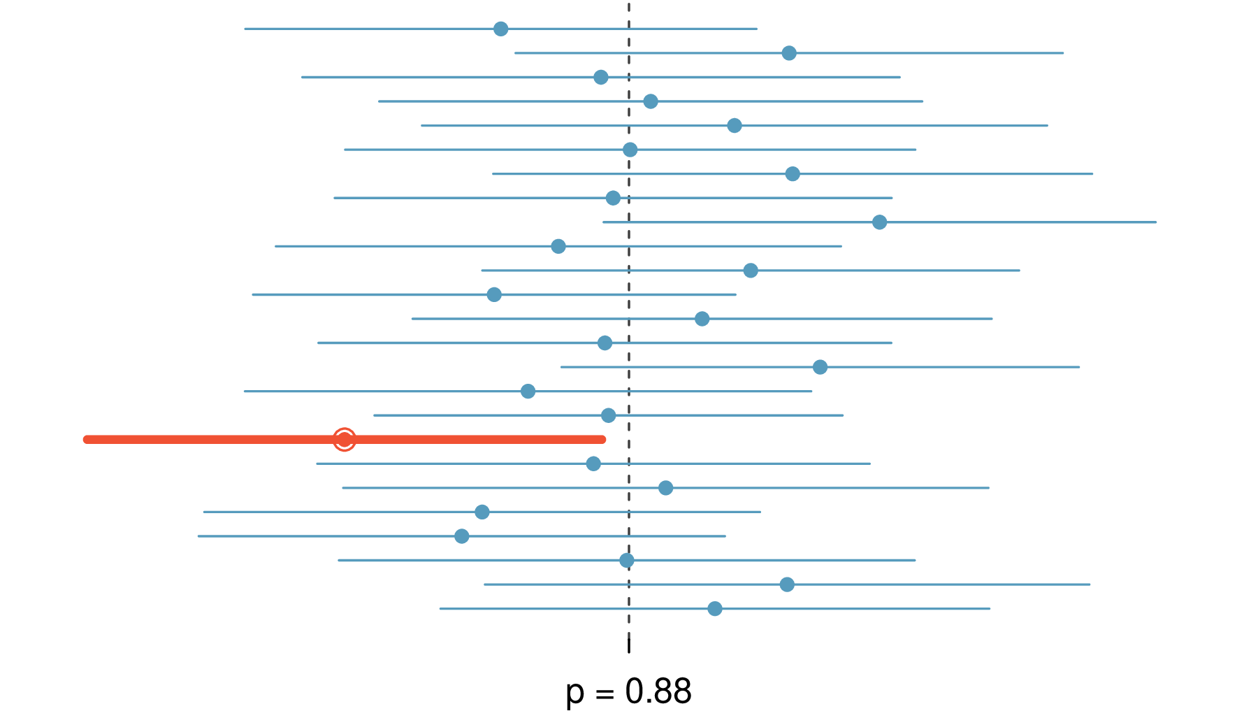
Twenty-five point estimates and confidence intervals from the simulations are shown. These intervals are shown relative to the population proportion p equals 0.88. The point estimates vary around the true population proportion of 0.88, but most of their confidence intervals overlap the value p equals 0.88. One of the 25 intervals does not have a confidence interval that overlaps the population proportion, and this interval has been bolded. We might say that this confidence interval did not capture the parameter p equals 0.88. — Figure 5.2.2. Twenty-five point estimates and confidence intervals from the simulations in Subsection 5.1.2. These intervals are shown relative to the population proportion \(p = 0.88\text{.}\) Only 1 of these 25 intervals did not capture the population proportion, and this interval has been bolded.
🔗

Example 5.2.3. Interpreting when an interval doesn’t capture the parameter.

In Figure 5.2.2, one interval does not contain \(p = 0.88\text{.}\) Does this imply that the population proportion used in the simulation could not have been \(p = 0.88\text{?}\)

🔗

Solution.

Just as some observations naturally occur more than 1.96 standard deviations from the mean, some point estimates will be more than 1.96 standard errors from the parameter of interest. A confidence interval only provides a plausible range of values. While we might say other values are implausible based on the data, this does not mean they are impossible.

🔗

Subsection 5.2.2 Constructing a 95% Confidence Interval

Our sample proportion \(\hat{p}\) is the most plausible value of the population proportion, so it makes sense to build a confidence interval around this point estimate. The standard error provides a guide for how large we should make the confidence interval.

🔗

The standard error represents the standard deviation of the point estimate, and when the Central Limit Theorem conditions are satisfied, the point estimate closely follows a normal distribution. In a normal distribution, 95% of the data is within 1.96 standard deviations of the mean. Using this principle, we can construct a confidence interval that extends 1.96 standard errors from the sample proportion to be 95% confident that the interval captures the population proportion:

🔗

\begin{align*} \text{point estimate}\ \amp\pm\ 1.96 \times SE\\ \hat{p}\ \amp\pm\ 1.96 \times \sqrt{\frac{p (1 - p)}{n}} \end{align*}

But what does “95% confident” mean? Suppose we took many samples and built a 95% confidence interval from each. Then about 95% of those intervals would contain the parameter, \(p\text{.}\) Figure 5.2.2 shows the process of creating 25 intervals from 25 samples from the simulation in Subsection 5.1.2, where 24 of the resulting confidence intervals contain the simulation’s population proportion of \(p = 0.88\text{,}\) and one interval does not.

🔗

95% confidence interval for a parameter.

When the distribution of a point estimate qualifies for the Central Limit Theorem and therefore closely follows a normal distribution, we can construct a 95% confidence interval as

🔗

Example 5.2.4. 95% CI for solar energy support.

In Section 5.1 we learned about a Pew Research poll where 88.7% of a random sample of 1,000 American adults supported expanding the role of solar power. Compute and interpret a 95% confidence interval for the population proportion.

🔗

Solution.

We earlier confirmed that \(\hat{p}\) follows a normal distribution and has a standard error of \(SE_{\hat{p}} = 0.0100\text{.}\) To compute the 95% confidence interval, plug the point estimate \(\hat{p} = 0.887\) and standard error into the 95% confidence interval formula:

🔗

\begin{align*} \hat{p} \pm 1.96 \times SE_{\hat{p}} \amp\quad\to\quad 0.887 \pm 1.96 \times 0.0100\\ \amp\quad\to\quad (0.8674, 0.9066) \end{align*}

We are 95% confident that the actual proportion of American adults who support expanding solar power is between 86.7% and 90.7%. (It’s common to round to the nearest percentage point or nearest tenth of a percentage point when reporting a confidence interval.)

🔗

Subsection 5.2.3 Changing the Confidence Level

Suppose we want to consider confidence intervals where the confidence level is higher than 95%, such as a confidence level of 99%. Think back to the analogy about trying to catch a fish: if we want to be more sure that we will catch the fish, we should use a wider net. To create a 99% confidence level, we must also widen our 95% interval. On the other hand, if we want an interval with lower confidence, such as 90%, we could use a slightly narrower interval than our original 95% interval.

🔗

The 95% confidence interval structure provides guidance in how to make intervals with different confidence levels. The general 95% confidence interval for a point estimate that follows a normal distribution is

🔗

\begin{align*} \text{point estimate}\ \amp\pm\ 1.96 \times SE \end{align*}

There are three components to this interval: the point estimate, “1.96”, and the standard error. The choice of \(1.96\times SE\) was based on capturing 95% of the data since the estimate is within 1.96 standard errors of the parameter about 95% of the time. The choice of 1.96 corresponds to a 95% confidence level.

🔗

Checkpoint 5.2.5.

If \(X\) is a normally distributed random variable, what is the probability of the value \(X\) being within 2.58 standard deviations of the mean?

🔗

Solution.

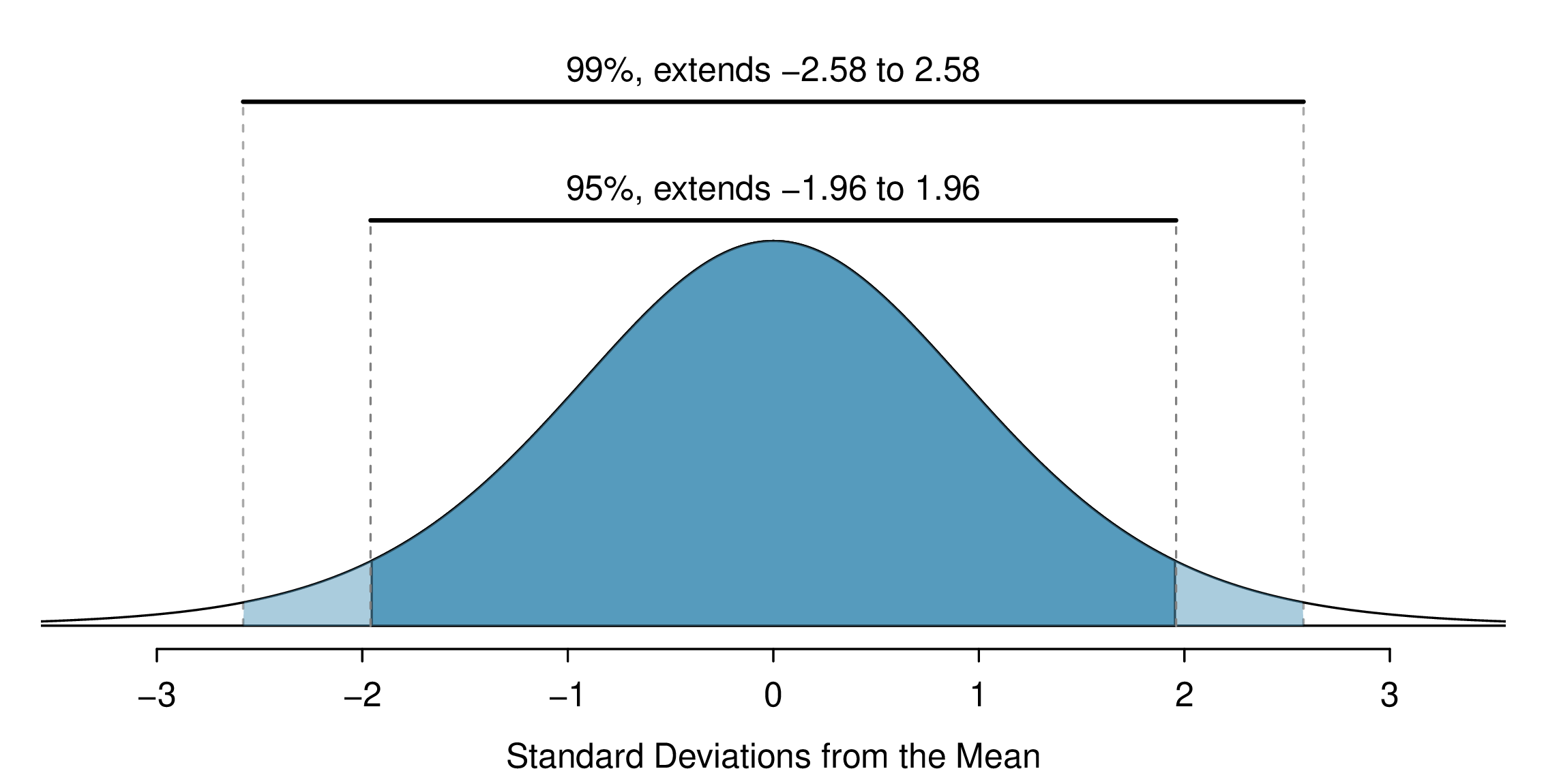
This is equivalent to asking how often the Z-score will be larger than -2.58 but less than 2.58. For a picture, see Figure 5.2.6. To determine this probability, we can use statistical software, a calculator, or a table to look up -2.58 and 2.58 for a normal distribution: 0.0049 and 0.9951. Thus, there is a \(0.9951-0.0049 \approx 0.99\) probability that an unobserved normal random variable \(X\) will be within 2.58 standard deviations of \(\mu\text{.}\)

🔗

This exercise highlights that 99% of the time a normal random variable will be within 2.58 standard deviations of the mean. To create a 99% confidence interval, change 1.96 in the 95% confidence interval formula to be 2.58. That is, the formula for a 99% confidence interval is

🔗

\begin{align*} \text{point estimate}\ \amp\pm\ 2.58 \times SE \end{align*}

A standard normal distribution is shown, where standard is the term used to indicate that the normal distribution is centered at 0 and has a standard deviation of 1. Portions of the normal distribution have been shaded. First, the central 95% portion of the distribution has been shaded in a dark blue, and this region has an annotation stating 95%, extends from -1.96 to 1.96. Recall that the value of 1.96 closely matches our 68-95-99.7 rule for the normal distribution, which had stated that about 95% of the area under the normal distribution lied within 2 standard deviations of the mean. Second, a slightly broader region of the normal distribution is shaded, in this case from about -2.5 to positive 2.5, and this has an annotation stating, 99%, extends -2.58 to 2.58. The values described here -- 1.96 and 2.58 -- are the z-star values that we would use for 95% and 99% confidence intervals, respectively. — Figure 5.2.6. The area between \(-z^{\star}\) and \(z^{\star}\) increases as \(z^{\star}\) becomes larger. If the confidence level is 99%, we choose \(z^{\star}\) such that 99% of a normal normal distribution is between \(-z^{\star}\) and \(z^{\star}\text{,}\) which corresponds to 0.5% in the lower tail and 0.5% in the upper tail: \(z^{\star}=2.58\text{.}\)
🔗

This approach -- using the Z-scores in the normal model to compute confidence levels -- is appropriate when a point estimate such as \(\hat{p}\) is associated with a normal distribution. For some other point estimates, a normal model is not a good fit; in these cases, we’ll use alternative distributions that better represent the sampling distribution.

🔗

Confidence interval using any confidence level.

If a point estimate closely follows a normal model with standard error \(SE\text{,}\) then a confidence interval for the population parameter is

🔗

where \(z^{\star}\) corresponds to the confidence level selected.

🔗

Figure 5.2.6 provides a picture of how to identify \(z^{\star}\) based on a confidence level. We select \(z^{\star}\) so that the area between \(-z^{\star}\) and \(z^{\star}\) in the standard normal distribution, \(N(0, 1)\text{,}\) corresponds to the confidence level.

🔗

Margin of error.

In a confidence interval, \(z^{\star}\times SE\) is called the margin of error.

🔗

Example 5.2.7. 90% CI for solar energy support.

Use the data in Example 5.2.4 to create a 90% confidence interval for the proportion of American adults that support expanding the use of solar power. We have already verified conditions for normality.

🔗

Solution.

We first find \(z^{\star}\) such that 90% of the distribution falls between \(-z^{\star}\) and \(z^{\star}\) in the standard normal distribution, \(N(\mu = 0, \sigma = 1)\text{.}\) We can do this using a graphing calculator, statistical software, or a probability table by looking for an upper tail of 5% (the other 5% is in the lower tail): \(z^{\star}=1.65\text{.}\) The 90% confidence interval can then be computed as

🔗

\begin{align*} \hat{p}\ \amp\pm\ 1.6449 \times SE_{\hat{p}}\\ \amp\quad\to\quad 0.887\ \pm\ 1.65 \times 0.0100\\ \amp\quad\to\quad (0.8705, 0.9034) \end{align*}

That is, we are 90% confident that 87.1% to 90.3% of American adults supported the expansion of solar power in 2018.

🔗

Subsection 5.2.4 More Case Studies

In New York City on October 23rd, 2014, a doctor who had recently been treating Ebola patients in Guinea went to the hospital with a slight fever and was subsequently diagnosed with Ebola. Soon thereafter, an NBC 4 New York/The Wall Street Journal/Marist Poll found that 82% of New Yorkers favored a “mandatory 21-day quarantine for anyone who has come in contact with an Ebola patient”. This poll included responses of 1,042 New York adults between Oct 26th and 28th, 2014.

🔗

Example 5.2.8.

What is the point estimate in this case, and is it reasonable to use a normal distribution to model that point estimate?

🔗

Solution.

The point estimate, based on a sample of size \(n = 1042\text{,}\) is \(\hat{p} = 0.82\text{.}\) To check whether \(\hat{p}\) can be reasonably modeled using a normal distribution, we check independence (the poll is based on a simple random sample) and the success-failure condition (\(1042 \times \hat{p} \approx 854\) and \(1042 \times (1 - \hat{p}) \approx 188\text{,}\) both easily greater than 10). With the conditions met, we are assured that the sampling distribution of \(\hat{p}\) can be reasonably modeled using a normal distribution.

🔗

Example 5.2.9.

Estimate the standard error of \(\hat{p} = 0.82\) from the Ebola survey.

🔗

Solution.

We’ll use the substitution approximation of \(p \approx \hat{p} = 0.82\) to compute the standard error:

🔗

\begin{align*} SE_{\hat{p}} \amp= \sqrt{\frac{p(1-p)}{n}}\\ \amp\approx \sqrt{\frac{0.82 (1 - 0.82)}{1042}}\\ \amp= 0.012 \end{align*}

🔗

Example 5.2.10.

Construct a 95% confidence interval for \(p\text{,}\) the proportion of New York adults who supported a quarantine for anyone who has come into contact with an Ebola patient.

🔗

Solution.

Using the standard error \(SE = 0.012\) from the previous example, the point estimate 0.82, and \(z^{\star} = 1.96\) for a 95% confidence level, the confidence interval is

🔗

\begin{align*} \text{point estimate} \ \amp\pm\ z^{\star} \times SE\\ \amp\quad\to\quad 0.82 \ \pm\ 1.96\times 0.012\\ \amp\quad\to\quad (0.796, 0.844) \end{align*}

We are 95% confident that the proportion of New York adults in October 2014 who supported a quarantine for anyone who had come into contact with an Ebola patient was between 0.796 and 0.844.

🔗

Checkpoint 5.2.11.

Answer the following two questions about the confidence interval from the example above:

🔗

What does 95% confident mean in this context?

🔗
Do you think the confidence interval is still valid for the opinions of New Yorkers today?

🔗

Solution.

If we took many such samples and computed a 95% confidence interval for each, then about 95% of those intervals would contain the actual proportion of New York adults who supported a quarantine for anyone who has come into contact with an Ebola patient.
🔗

🔗
Not necessarily. The poll was taken at a time where there was a huge public safety concern. Now that people have had some time to step back, they may have changed their opinions. We would need to run a new poll if we wanted to get an estimate of the current proportion of New York adults who would support such a quarantine period.
🔗

🔗

🔗

Checkpoint 5.2.12.

In the Pew Research poll about solar energy, they also inquired about other forms of energy, and 84.8% of the 1,000 respondents supported expanding the use of wind turbines.

🔗

Is it reasonable to model the proportion of US adults who support expanding wind turbines using a normal distribution?

🔗
Create a 99% confidence interval for the level of American support for expanding the use of wind turbines for power generation.

🔗

Solution.

The survey was a random sample and counts are both \(\geq 10\) (\(1000 \times 0.848 = 848\) and \(1000 \times 0.152 = 152\)), so independence and the success-failure condition are satisfied, and \(\hat{p} = 0.848\) can be modeled using a normal distribution.
🔗

🔗
We already confirmed that \(\hat{p}\) closely follows a normal distribution, so we can use the C.I. formula:
🔗

\begin{align*} \text{point estimate} \amp\pm z^{\star} \times SE \end{align*}

In this case, the point estimate is \(\hat{p} = 0.848\text{.}\) For a 99% confidence interval, \(z^{\star} = 2.58\text{.}\) Computing the standard error: \(SE_{\hat{p}} = \sqrt{\frac{0.848(1 - 0.848)} {1000}} = 0.0114\text{.}\) Finally, we compute the interval as \(0.848 \pm 2.58 \times 0.0114 \to (0.8186, 0.8774)\text{.}\) It is also important to always provide an interpretation for the interval: we are 99% confident the proportion of American adults that support expanding the use of wind turbines in 2018 is between 81.9% and 87.7%.
🔗

🔗

🔗

We can also construct confidence intervals for other parameters, such as a population mean. In these cases, a confidence interval would be computed in a similar way to that of a single proportion: a point estimate plus/minus some margin of error. We’ll dive into these details in later chapters.

🔗

Confidence interval for a single proportion.

Once you’ve determined a one-proportion confidence interval would be helpful for an application, there are four steps to constructing the interval:

Prepare. 🔗: Identify \(\hat{p}\) and \(n\text{,}\) and determine what confidence level you wish to use.
🔗
Check. 🔗: Verify the conditions to ensure \(\hat{p}\) is nearly normal. For one-proportion confidence intervals, use \(\hat{p}\) in place of \(p\) to check the success-failure condition.
🔗
Calculate. 🔗: If the conditions hold, compute \(SE\) using \(\hat{p}\text{,}\) find \(z^{\star}\text{,}\) and construct the interval.
🔗
Conclude. 🔗: Interpret the confidence interval in the context of the problem.
🔗

🔗

Subsection 5.2.5 Interpreting Confidence Intervals

In each of the examples, we described the confidence intervals by putting them into the context of the data and also using somewhat formal language:

🔗

Solar. 🔗: We are 90% confident that 87.1% to 90.4% of American adults support the expansion of solar power in 2018.
🔗
Ebola. 🔗: We are 95% confident that the proportion of New York adults in October 2014 who supported a quarantine for anyone who had come into contact with an Ebola patient was between 0.796 and 0.844.
🔗
Wind Turbine. 🔗: We are 99% confident the proportion of Americans adults that support expanding the use of wind turbines is between 81.9% and 87.7% in 2018.
🔗

First, notice that the statements are always about the population parameter, which considers all American adults for the energy polls or all New York adults for the quarantine poll.

🔗

We also avoided another common mistake: incorrect language might try to describe the confidence interval as capturing the population parameter with a certain probability. Making a probability interpretation is a common error: while it might be useful to think of it as a probability, the confidence level only quantifies how plausible it is that the parameter is in the given interval.

🔗

Another important consideration of confidence intervals is that they are only about the population parameter. A confidence interval says nothing about individual observations or point estimates. Confidence intervals only provide a plausible range for population parameters.

🔗

Lastly, keep in mind the methods we discussed only apply to sampling error, not to bias. If a data set is collected in a way that will tend to systematically under-estimate (or over-estimate) the population parameter, the techniques we have discussed will not address that problem. Instead, we rely on careful data collection procedures to help protect against bias in the examples we have considered, which is a common practice employed by data scientists to combat bias.

🔗

Checkpoint 5.2.13.

Consider the 90% confidence interval for the solar energy survey: 87.1% to 90.4%. If we ran the survey again, can we say that we’re 90% confident that the new survey’s proportion will be between 87.1% and 90.4%?

🔗

Solution.

No, a confidence interval only provides a range of plausible values for a parameter, not future point estimates.

🔗

Exercises 5.2.6 Section 5.2 Exercises

1. Chronic illness, Part I..

In 2013, the Pew Research Foundation reported that "45% of U.S. adults report that they live with one or more chronic conditions". However, this value was based on a sample, so it may not be a perfect estimate for the population parameter of interest on its own. The study reported a standard error of about 1.2%, and a normal model may reasonably be used in this setting. Create a 95% confidence interval for the proportion of U.S. adults who live with one or more chronic conditions. Also interpret the confidence interval in the context of the study.

🔗

2. Twitter users and news. Part I..

A poll conducted in 2013 found that 52% of U.S. adult Twitter users get at least some news on Twitter. The standard error for this estimate was 2.4%, and a normal distribution may be used to model the sample proportion. Construct a 99% confidence interval for the fraction of U.S. adult Twitter users who get some news on Twitter, and interpret the confidence interval in context.

🔗

3. Chronic illness, Part II..

In 2013, the Pew Research Foundation reported that "45% of U.S. adults report that they live with one or more chronic conditions", and the standard error for this estimate is 1.2%. Identify each of the following statements as true or false. Provide an explanation to justify each of your answers.

🔗

We can say with certainty that the confidence interval from the chronic illness exercise contains the true percentage of U.S. adults who suffer from a chronic illness.

🔗
If we repeated this study 1,000 times and constructed a 95% confidence interval for each study, then approximately 950 of those confidence intervals would contain the true fraction of U.S. adults who suffer from chronic illnesses.

🔗
The poll provides statistically significant evidence (at the \(\alpha = 0.05\) level) that the percentage of U.S. adults who suffer from chronic illnesses is below 50%.

🔗
Since the standard error is 1.2%, only 1.2% of people in the study communicated uncertainty about their answer.

🔗

🔗

4. Twitter users and news, Part II..

A poll conducted in 2013 found that 52% of U.S. adult Twitter users get at least some news on Twitter, and the standard error for this estimate was 2.4%. Identify each of the following statements as true or false. Provide an explanation to justify each of your answers.

🔗

The data provide statistically significant evidence that more than half of U.S. adult Twitter users get some news through Twitter. Use a significance level of \(\alpha = 0.01\text{.}\) (This part uses concepts from Section 5.3 and will be corrected in a future edition.)

🔗
Since the standard error is 2.4%, we can conclude that 97.6% of all U.S. adult Twitter users were included in the study.

🔗
If we want to reduce the standard error of the estimate, we should collect less data.

🔗
If we construct a 90% confidence interval for the percentage of U.S. adult Twitter users who get some news through Twitter, this confidence interval will be wider than a corresponding 99% confidence interval.

🔗

🔗

5. Waiting at an ER, Part I..

A hospital administrator hoping to improve wait times decides to estimate the average emergency room waiting time at her hospital. She collects a simple random sample of 64 patients and determines the time (in minutes) between when they checked in to the ER until they were first seen by a doctor. A 95% confidence interval based on this sample is (128 minutes, 147 minutes), which is based on the normal model for the mean. Determine whether the following statements are true or false, and explain your reasoning.

🔗

We are 95% confident that the average waiting time of these 64 emergency room patients is between 128 and 147 minutes.

🔗
We are 95% confident that the average waiting time of all patients at this hospital’s emergency room is between 128 and 147 minutes.

🔗
95% of random samples have a sample mean between 128 and 147 minutes.

🔗
A 99% confidence interval would be narrower than the 95% confidence interval since we need to be more sure of our estimate.

🔗
The margin of error is 9.5 and the sample mean is 137.5.

🔗
In order to decrease the margin of error of a 95% confidence interval to half of what it is now, we would need to double the sample size. (Hint: the margin of error for a mean scales in the same way with sample size as the margin of error for a proportion.)

🔗

🔗

6. Mental health..

The General Social Survey asked the question: "For how many days during the past 30 days was your mental health, which includes stress, depression, and problems with emotions, not good?" Based on responses from 1,151 US residents, the survey reported a 95% confidence interval of 3.40 to 4.24 days in 2010.

🔗

Interpret this interval in context of the data.

🔗
What does "95% confident" mean? Explain in the context of the application.

🔗
Suppose the researchers think a 99% confidence level would be more appropriate for this interval. Will this new interval be smaller or wider than the 95% confidence interval?

🔗
If a new survey were to be done with 500 Americans, do you think the standard error of the estimate would be larger, smaller, or about the same.

🔗

🔗

7. Website registration.

A website is trying to increase registration for first-time visitors, exposing 1% of these visitors to a new site design. Of 752 randomly sampled visitors over a month who saw the new design, 64 registered.

🔗

Check any conditions required for constructing a confidence interval.

🔗
Compute the standard error.

🔗
Construct and interpret a 90% confidence interval for the fraction of first-time visitors of the site who would register under the new design (assuming stable behaviors by new visitors over time).

🔗

🔗

8. Coupons driving visits.

A store randomly samples 603 shoppers over the course of a year and finds that 142 of them made their visit because of a coupon they’d received in the mail. Construct a 95% confidence interval for the fraction of all shoppers during the year whose visit was because of a coupon they’d received in the mail.

🔗

Prev Top Next