Binomial distribution

Section 4.3 Binomial distribution

The binomial distribution is used to describe the number of successes in a fixed number of trials. This is different from the geometric distribution, which described the number of trials we must wait before we observe a success.

🔗

Subsection 4.3.1 The binomial distribution

Let’s again imagine ourselves back at the insurance agency where 70% of individuals do not exceed their deductible.

🔗

Example 4.3.1. Probability of one exceeding deductible.

Suppose the insurance agency is considering a random sample of four individuals they insure. What is the chance exactly one of them will exceed the deductible and the other three will not? Let’s call the four people Ariana (\(A\)), Brittany (\(B\)), Carlton (\(C\)), and Damian (\(D\)) for convenience.

🔗

Solution.

Let’s consider a scenario where one person exceeds the deductible:

\begin{align*} \amp P(A=\text{exceed}, B=\text{not}, C=\text{not}, D=\text{not})\\ \amp \quad = P(A=\text{exceed}) \cdot P(B=\text{not}) \cdot P(C=\text{not}) \cdot P(D=\text{not})\\ \amp \quad = (0.3)(0.7)(0.7)(0.7)\\ \amp \quad = (0.7)^3 (0.3)^1\\ \amp \quad = 0.103 \end{align*}

But there are three other scenarios: Brittany, Carlton, or Damian could have been the one to exceed the deductible. In each of these cases, the probability is again \((0.7)^3(0.3)^1\text{.}\) These four scenarios exhaust all the possible ways that exactly one of these four people could have exceeded the deductible, so the total probability is

\begin{equation*} 4 \times (0.7)^3(0.3)^1 = 0.412 \end{equation*}

🔗

Checkpoint 4.3.2.

Verify that the scenario where Brittany is the only one to exceed the deductible has probability \((0.7)^3(0.3)^1\text{.}\)

🔗

Solution.

\(P(A=\text{not}, B=\text{exceed}, C=\text{not}, D=\text{not}) = (0.7)(0.3)(0.7)(0.7) = (0.7)^3(0.3)^1\text{.}\)

🔗

The scenario outlined in Example 4.3.1 is an example of a binomial distribution scenario. The binomial distribution describes the probability of having exactly \(k\) successes in \(n\) independent Bernoulli trials with probability of a success \(p\) (in Example 4.3.1, \(n=4\text{,}\) \(k=3\text{,}\) \(p=0.7\)). We would like to determine the probabilities associated with the binomial distribution more generally, i.e. we want a formula where we can use \(n\text{,}\) \(k\text{,}\) and \(p\) to obtain the probability. To do this, we reexamine each part of Example 4.3.1.

🔗

There were four individuals who could have been the one to exceed the deductible, and each of these four scenarios had the same probability. Thus, we could identify the final probability as

\begin{equation*} [\text{number of scenarios}] \times P(\text{single scenario}) \end{equation*}

The first component of this equation is the number of ways to arrange the \(k=3\) successes among the \(n=4\) trials. The second component is the probability of any of the four (equally probable) scenarios.

🔗

Consider \(P(\text{single scenario})\) under the general case of \(k\) successes and \(n-k\) failures in the \(n\) trials. In any such scenario, we apply the Multiplication Rule for independent events:

\begin{equation*} p^k(1-p)^{n-k} \end{equation*}

This is our general formula for \(P(\text{single scenario})\text{.}\)

🔗

Secondly, we introduce a general formula for the number of ways to choose \(k\) successes in \(n\) trials, i.e. arrange \(k\) successes and \(n-k\) failures:

\begin{equation*} \binom{n}{k} = \frac{n!}{k!(n-k)!} \end{equation*}

The quantity \(\binom{n}{k}\) is read n choose k.

Other notation for \(n\) choose \(k\) includes \(_nC_k\text{,}\) \(C_n^k\text{,}\) and \(C(n,k)\text{.}\)

The exclamation point notation (e.g. \(k!\)) denotes a factorial expression.

\begin{align*} 0! \amp = 1\\ 1! \amp = 1\\ 2! \amp = 2\times 1 = 2\\ 3! \amp = 3\times 2\times 1 = 6\\ 4! \amp = 4\times 3\times 2\times 1 = 24\\ \amp \vdots\\ n! \amp = n\times(n-1)\times\cdots\times 3\times 2\times 1 \end{align*}

Using the formula, we can compute the number of ways to choose \(k=3\) successes in \(n=4\) trials:

\begin{equation*} \binom{4}{3} = \frac{4!}{3!(4-3)!} = \frac{4!}{3!1!} = \frac{4\times 3\times 2\times 1}{(3\times 2\times 1)(1)} = 4 \end{equation*}

This result is exactly what we found by carefully thinking of each possible scenario in Example 4.3.1.

🔗

Substituting \(n\) choose \(k\) for the number of scenarios and \(p^k(1-p)^{n-k}\) for the single scenario probability yields the general binomial formula.

🔗

Binomial distribution
🔗

Suppose the probability of a single trial being a success is \(p\text{.}\) Then the probability of observing exactly \(k\) successes in \(n\) independent trials is given by

\begin{equation*} \binom{n}{k}p^k(1-p)^{n-k} = \frac{n!}{k!(n-k)!}p^k(1-p)^{n-k} \end{equation*}

The mean, variance, and standard deviation of the number of observed successes are

\begin{align*} \mu \amp = np \amp \sigma^2 \amp = np(1-p) \amp \sigma \amp = \sqrt{np(1-p)} \end{align*}

🔗

🔗

Is it binomial? Four conditions to check.
🔗

The trials are independent.
🔗

🔗

The number of trials, \(n\text{,}\) is fixed.
🔗

🔗

Each trial outcome can be classified as a success or failure.
🔗

🔗

The probability of a success, \(p\text{,}\) is the same for each trial.
🔗

🔗

🔗

🔗

Example 4.3.3. Probability of 3 of 8 exceeding deductible.

What is the probability that 3 of 8 randomly selected individuals will have exceeded the insurance deductible, i.e. that 5 of 8 will not exceed the deductible? Recall that 70% of individuals will not exceed the deductible.

🔗

Solution.

We would like to apply the binomial model, so we check the conditions. The number of trials is fixed (\(n=8\)) (condition 2) and each trial outcome can be classified as a success or failure (condition 3). Because the sample is random, the trials are independent (condition 1) and the probability of a success is the same for each trial (condition 4).

🔗

In the outcome of interest, there are \(k=5\) successes in \(n=8\) trials (recall that a success is an individual who does not exceed the deductible), and the probability of a success is \(p=0.7\text{.}\) So the probability that 5 of 8 will not exceed the deductible and 3 will exceed the deductible is given by

\begin{align*} \binom{8}{5}(0.7)^5(1-0.7)^{8-5} \amp = \frac{8!}{5!(8-5)!}(0.7)^5(1-0.7)^{8-5}\\ \amp = \frac{8!}{5!3!}(0.7)^5(0.3)^3 \end{align*}

Dealing with the factorial part:

\begin{equation*} \frac{8!}{5!3!} = \frac{8\times 7\times 6\times 5\times 4\times 3\times 2\times 1}{(5\times 4\times 3\times 2\times 1)(3\times 2\times 1)} = \frac{8\times 7\times 6}{3\times 2\times 1} = 56 \end{equation*}

Using \((0.7)^5(0.3)^3 \approx 0.00454\text{,}\) the final probability is about \(56 \times 0.00454 \approx 0.254\text{.}\)

🔗

Computing binomial probabilities
🔗

The first step in using the binomial model is to check that the model is appropriate. The second step is to identify \(n\text{,}\) \(p\text{,}\) and \(k\text{.}\) As the last stage use software or the formulas to determine the probability, then interpret the results.
🔗

If you must do calculations by hand, it’s often useful to cancel out as many terms as possible in the top and bottom of the binomial coefficient.
🔗

🔗

Checkpoint 4.3.4.

If we randomly sampled 40 case files from the insurance agency discussed earlier, how many of the cases would you expect to not have exceeded the deductible in a given year? What is the standard deviation of the number that would not have exceeded the deductible?

🔗

Solution.

We are asked to determine the expected number (the mean) and the standard deviation, both of which can be directly computed from the formulas: \(\mu = np = 40 \times 0.7 = 28\) and \(\sigma = \sqrt{np(1-p)} = \sqrt{40 \times 0.7 \times 0.3} = 2.9\text{.}\) Because very roughly 95% of observations fall within 2 standard deviations of the mean (see Section 1.6.3), we would probably observe at least 22 but fewer than 34 individuals in our sample who would not exceed the deductible.

🔗

Checkpoint 4.3.5.

The probability that a random smoker will develop a severe lung condition in his or her lifetime is about 0.3. If you have 4 friends who smoke, are the conditions for the binomial model satisfied?

🔗

Solution.

One possible answer: if the friends know each other, then the independence assumption is probably not satisfied. For example, acquaintances may have similar smoking habits, or those friends might make a pact to quit together.

🔗

Checkpoint 4.3.6.

Suppose these four friends do not know each other and we can treat them as if they were a random sample from the population. Is the binomial model appropriate? What is the probability that

None of them will develop a severe lung condition?
🔗

🔗
One will develop a severe lung condition?
🔗

🔗
That no more than one will develop a severe lung condition?
🔗

🔗

🔗

Solution.

To check if the binomial model is appropriate, we must verify the conditions. (i) Since we are supposing we can treat the friends as a random sample, they are independent. (ii) We have a fixed number of trials (\(n=4\)). (iii) Each outcome is a success or failure. (iv) The probability of a success is the same for each trial since the individuals are like a random sample (\(p=0.3\) if we say a “success” is someone getting a lung condition, a morbid choice).

🔗

Compute parts (a) and (b) using the binomial formula: \(P(0) = \binom{4}{0}(0.3)^0(0.7)^4 = 1 \times 1 \times 0.7^4 = 0.2401\text{,}\) \(P(1) = \binom{4}{1}(0.3)^1(0.7)^3 = 0.4116\text{.}\) Note: \(0! = 1\text{.}\) Part (c) can be computed as the sum of parts (a) and (b): \(P(0) + P(1) = 0.2401 + 0.4116 = 0.6517\text{.}\) That is, there is about a 65% chance that no more than one of your four smoking friends will develop a severe lung condition.

🔗

Checkpoint 4.3.7.

What is the probability that at least 2 of your 4 smoking friends will develop a severe lung condition in their lifetimes?

🔗

Solution.

The complement (no more than one will develop a severe lung condition) as computed in Checkpoint 4.3.6 as 0.6517, so we compute one minus this value: 0.3483.

🔗

Checkpoint 4.3.8.

Suppose you have 7 friends who are smokers and they can be treated as a random sample of smokers.

How many would you expect to develop a severe lung condition, i.e. what is the mean?
🔗

🔗
What is the probability that at most 2 of your 7 friends will develop a severe lung condition?
🔗

🔗

🔗

Solution.

(a) \(\mu = 0.3 \times 7 = 2.1\text{.}\) (b) \(P(\text{0, 1, or 2 develop severe lung condition}) = P(k=0) + P(k=1) + P(k=2) = 0.6471\text{.}\)

🔗

Next we consider the first term in the binomial probability, \(n\) choose \(k\) under some special scenarios.

🔗

Checkpoint 4.3.9.

Why is it true that \(\binom{n}{0} = 1\) and \(\binom{n}{n} = 1\) for any number \(n\text{?}\)

🔗

Solution.

Frame these expressions into words. How many different ways are there to arrange 0 successes and \(n\) failures in \(n\) trials? (1 way.) How many different ways are there to arrange \(n\) successes and 0 failures in \(n\) trials? (1 way.)

🔗

Checkpoint 4.3.10.

How many ways can you arrange one success and \(n-1\) failures in \(n\) trials? How many ways can you arrange \(n-1\) successes and one failure in \(n\) trials?

🔗

Solution.

One success and \(n-1\) failures: there are exactly \(n\) unique places we can put the success, so there are \(n\) ways to arrange one success and \(n-1\) failures. A similar argument is used for the second question. Mathematically, we show these results by verifying the following two equations:

\begin{equation*} \binom{n}{1} = n, \qquad \binom{n}{n-1} = n \end{equation*}

🔗

Subsection 4.3.2 Normal approximation to the binomial distribution

The binomial formula is cumbersome when the sample size (\(n\)) is large, particularly when we consider a range of observations. In some cases we may use the normal distribution as an easier and faster way to estimate binomial probabilities.

🔗

Example 4.3.11. Smoker survey probability.

Approximately 15% of the US population smokes cigarettes. A local government believed their community had a lower smoker rate and commissioned a survey of 400 randomly selected individuals. The survey found that only 42 of the 400 participants smoke cigarettes. If the true proportion of smokers in the community was really 15%, what is the probability of observing 42 or fewer smokers in a sample of 400 people?

🔗

Solution.

We leave the usual verification that the four conditions for the binomial model are valid as an exercise.

🔗

The question posed is equivalent to asking, what is the probability of observing \(k=0\text{,}\) 1, 2, …, or 42 smokers in a sample of \(n=400\) when \(p=0.15\text{?}\) We can compute these 43 different probabilities and add them together to find the answer:

\begin{align*} \amp P(k=0 \text{ or } k=1 \text{ or } \cdots \text{ or } k=42)\\ \amp \quad = P(k=0) + P(k=1) + \cdots + P(k=42)\\ \amp \quad = 0.0054 \end{align*}

If the true proportion of smokers in the community is \(p=0.15\text{,}\) then the probability of observing 42 or fewer smokers in a sample of \(n=400\) is 0.0054.

🔗

The computations in Example 4.3.11 are tedious and long. In general, we should avoid such work if an alternative method exists that is faster, easier, and still accurate. Recall that calculating probabilities of a range of values is much easier in the normal model. We might wonder, is it reasonable to use the normal model in place of the binomial distribution? Surprisingly, yes, if certain conditions are met.

🔗

Checkpoint 4.3.12.

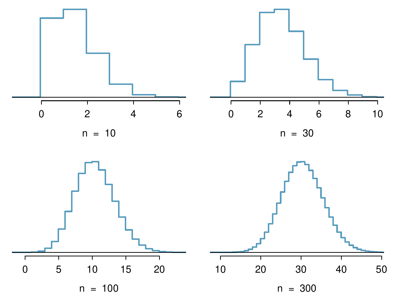
Here we consider the binomial model when the probability of a success is \(p=0.10\text{.}\) Figure 4.3.13 shows four hollow histograms for simulated samples from the binomial distribution using four different sample sizes: \(n=10, 30, 100, 300\text{.}\) What happens to the shape of the distributions as the sample size increases? What distribution does the last hollow histogram resemble?

🔗

Solution.

The distribution is transformed from a blocky and skewed distribution into one that rather resembles the normal distribution in last hollow histogram.

🔗

Figure 4.3.13. Hollow histograms of samples from the binomial model when \(p=0.10\text{.}\) The sample sizes for the four plots are \(n=10\text{,}\) 30, 100, and 300, respectively.
🔗

Normal approximation of the binomial distribution
🔗

The binomial distribution with probability of success \(p\) is nearly normal when the sample size \(n\) is sufficiently large that \(np\) and \(n(1-p)\) are both at least 10. The approximate normal distribution has parameters corresponding to the mean and standard deviation of the binomial distribution:

\begin{align*} \mu \amp = np \amp \sigma \amp = \sqrt{np(1-p)} \end{align*}

🔗

🔗

The normal approximation may be used when computing the range of many possible successes. For instance, we may apply the normal distribution to the setting of Example 4.3.11.

🔗

Example 4.3.14. Normal approximation for smoker survey.

How can we use the normal approximation to estimate the probability of observing 42 or fewer smokers in a sample of 400, if the true proportion of smokers is \(p=0.15\text{?}\)

🔗

Solution.

Showing that the binomial model is reasonable was a suggested exercise in Example 4.3.11. We also verify that both \(np\) and \(n(1-p)\) are at least 10:

\begin{align*} np \amp = 400 \times 0.15 = 60 \amp n(1-p) \amp = 400 \times 0.85 = 340 \end{align*}

With these conditions checked, we may use the normal approximation in place of the binomial distribution using the mean and standard deviation from the binomial model:

\begin{align*} \mu \amp = np = 60 \amp \sigma \amp = \sqrt{np(1-p)} = 7.14 \end{align*}

We want to find the probability of observing 42 or fewer smokers using this model.

🔗

Checkpoint 4.3.15.

Use the normal model \(N(\mu=60, \sigma=7.14)\) to estimate the probability of observing 42 or fewer smokers. Your answer should be approximately equal to the solution of Example 4.3.11: 0.0054.

🔗

Solution.

Compute the Z-score first: \(Z = \frac{42-60}{7.14} = -2.52\text{.}\) The corresponding left tail area is 0.0059.

🔗

Subsection 4.3.3 The normal approximation breaks down on small intervals

The normal approximation to the binomial distribution tends to perform poorly when estimating the probability of a small range of counts, even when the conditions are met.

🔗

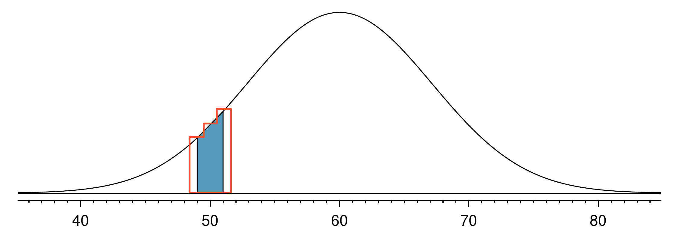
Suppose we wanted to compute the probability of observing 49, 50, or 51 smokers in 400 when \(p=0.15\text{.}\) With such a large sample, we might be tempted to apply the normal approximation and use the range 49 to 51. However, we would find that the binomial solution and the normal approximation notably differ:

\begin{align*} \text{Binomial:} \amp \text{ } 0.0649 \amp \text{Normal:} \amp \text{ } 0.0421 \end{align*}

We can identify the cause of this discrepancy using Figure 4.3.16, which shows the areas representing the binomial probability (outlined) and normal approximation (shaded). Notice that the width of the area under the normal distribution is 0.5 units too slim on both sides of the interval.

🔗

Figure 4.3.16. A normal curve with the area between 49 and 51 shaded. The outlined area represents the exact binomial probability.
🔗

Improving the normal approximation for the binomial distribution
🔗

The normal approximation to the binomial distribution for intervals of values is usually improved if cutoff values are modified slightly. The cutoff values for the lower end of a shaded region should be reduced by 0.5, and the cutoff value for the upper end should be increased by 0.5.
🔗

🔗

The tip to add extra area when applying the normal approximation is most often useful when examining a range of observations. In the example above, the revised normal distribution estimate is 0.0633, much closer to the exact value of 0.0649. While it is possible to also apply this correction when computing a tail area, the benefit of the modification usually disappears since the total interval is typically quite wide.

🔗

Exercises 4.3.4 Exercises

1. Underage drinking, Part I.

Data collected by the Substance Abuse and Mental Health Services Administration (SAMSHA) suggests that 69.7% of 18-20 year olds consumed alcoholic beverages in any given year.

Substance Abuse and Mental Health Services Administration, Results from the 2013 National Survey on Drug Use and Health: Summary of National Findings

🔗

Suppose a random sample of ten 18-20 year olds is taken. Is the use of the binomial distribution appropriate for calculating the probability that exactly six consumed alcoholic beverages? Explain.
🔗

🔗
Calculate the probability that exactly 6 out of 10 randomly sampled 18-20 year olds consumed an alcoholic drink.
🔗

🔗
What is the probability that exactly four out of ten 18-20 year olds have not consumed an alcoholic beverage?
🔗

🔗
What is the probability that at most 2 out of 5 randomly sampled 18-20 year olds have consumed alcoholic beverages?
🔗

🔗
What is the probability that at least 1 out of 5 randomly sampled 18-20 year olds have consumed alcoholic beverages?
🔗

🔗

🔗

2. Chickenpox, Part I.

Boston Children’s Hospital estimates that 90% of Americans have had chickenpox by the time they reach adulthood.

Boston Children’s Hospital, Chickenpox

🔗

Suppose we take a random sample of 100 American adults. Is the use of the binomial distribution appropriate for calculating the probability that exactly 97 out of 100 randomly sampled American adults had chickenpox during childhood? Explain.
🔗

🔗
Calculate the probability that exactly 97 out of 100 randomly sampled American adults had chickenpox during childhood.
🔗

🔗
What is the probability that exactly 3 out of a new sample of 100 American adults have not had chickenpox in their childhood?
🔗

🔗
What is the probability that at least 1 out of 10 randomly sampled American adults have had chickenpox?
🔗

🔗
What is the probability that at most 3 out of 10 randomly sampled American adults have not had chickenpox?
🔗

🔗

🔗

3. Underage drinking, Part II.

We learned in Exercise 4.3.4.1 that about 70% of 18-20 year olds consumed alcoholic beverages in any given year. We now consider a random sample of fifty 18-20 year olds.

🔗

How many people would you expect to have consumed alcoholic beverages? And with what standard deviation?
🔗

🔗
Would you be surprised if there were 45 or more people who have consumed alcoholic beverages?
🔗

🔗
What is the probability that 45 or more people in this sample have consumed alcoholic beverages? How does this probability relate to your answer to part (b)?
🔗

🔗

🔗

4. Chickenpox, Part II.

We learned in Exercise 4.3.4.2 that about 90% of American adults had chickenpox before adulthood. We now consider a random sample of 120 American adults.

🔗

How many people in this sample would you expect to have had chickenpox in their childhood? And with what standard deviation?
🔗

🔗
Would you be surprised if there were 105 people who have had chickenpox in their childhood?
🔗

🔗
What is the probability that 105 or fewer people in this sample have had chickenpox in their childhood? How does this probability relate to your answer to part (b)?
🔗

🔗

🔗

5. Game of dreidel.

A dreidel is a four-sided spinning top with the Hebrew letters nun, gimel, hei, and shin, one on each side. Each side is equally likely to come up in a single spin of the dreidel. Suppose you spin a dreidel three times. Calculate the probability of getting

🔗

at least one nun?
🔗

🔗
exactly 2 nuns?
🔗

🔗
exactly 1 hei?
🔗

🔗
at most 2 gimels?
🔗

🔗

🔗

6. Arachnophobia.

A Gallup Poll found that 7% of teenagers (ages 13 to 17) suffer from arachnophobia and are extremely afraid of spiders. At a summer camp there are 10 teenagers sleeping in each tent. Assume that these 10 teenagers are independent of each other.

⁴

Gallup Poll, Fear of Spiders

🔗

Calculate the probability that at least one of them suffers from arachnophobia.
🔗

🔗
Calculate the probability that exactly 2 of them suffer from arachnophobia.
🔗

🔗
Calculate the probability that at most 1 of them suffers from arachnophobia.
🔗

🔗
If the camp counselor wants to make sure no more than 1 teenager in each tent is afraid of spiders, does it seem reasonable for him to randomly assign teenagers to tents?
🔗

🔗

🔗

7. Eye color, Part II.

Exercise 4.2.12 introduces a husband and wife with brown eyes who have 0.75 probability of having children with brown eyes, 0.125 probability of having children with blue eyes, and 0.125 probability of having children with green eyes.

🔗

What is the probability that their first child will have green eyes and the second will not?
🔗

🔗
What is the probability that exactly one of their two children will have green eyes?
🔗

🔗
If they have six children, what is the probability that exactly two will have green eyes?
🔗

🔗
If they have six children, what is the probability that at least one will have green eyes?
🔗

🔗
What is the probability that the first green eyed child will be the 4th child?
🔗

🔗
Would it be considered unusual if only 2 out of their 6 children had brown eyes?
🔗

🔗

🔗

8. Sickle cell anemia.

Sickle cell anemia is a genetic blood disorder where red blood cells lose their flexibility and assume an abnormal, rigid, “sickle” shape, which results in a risk of various complications. If both parents are carriers of the disease, then a child has a 25% chance of having the disease, 50% chance of being a carrier, and 25% chance of neither having the disease nor being a carrier. If two parents who are carriers of the disease have 3 children, what is the probability that

🔗

two will have the disease?
🔗

🔗
none will have the disease?
🔗

🔗
at least one will neither have the disease nor be a carrier?
🔗

🔗
the first child with the disease will the be 3rd child?
🔗

🔗

🔗

9. Exploring permutations.

The formula for the number of ways to arrange \(n\) objects is \(n! = n \times (n-1) \times \cdots \times 2 \times 1\text{.}\) This exercise walks you through the derivation of this formula for a couple of special cases.

🔗

A small company has five employees: Anna, Ben, Carl, Damian, and Eddy. There are five parking spots in a row at the company, none of which are assigned, and each day the employees pull into a random parking spot. That is, all possible orderings of the cars in the row of spots are equally likely.

🔗

On a given day, what is the probability that the employees park in alphabetical order?
🔗

🔗
If the alphabetical order has an equal chance of occurring relative to all other possible orderings, how many ways must there be to arrange the five cars?
🔗

🔗
Now consider a sample of 8 employees instead. How many possible ways are there to order these 8 employees’ cars?
🔗

🔗

🔗

10. Male children.

While it is often assumed that the probabilities of having a boy or a girl are the same, the actual probability of having a boy is slightly higher at 0.51. Suppose a couple plans to have 3 kids.

🔗

Use the binomial model to calculate the probability that two of them will be boys.
🔗

🔗
Write out all possible orderings of 3 children, 2 of whom are boys. Use these scenarios to calculate the same probability from part (a) but using the addition rule for disjoint outcomes. Confirm that your answers from parts (a) and (b) match.
🔗

🔗
If we wanted to calculate the probability that a couple who plans to have 8 kids will have 3 boys, briefly describe why the approach from part (b) would be more tedious than the approach from part (a).
🔗

🔗

🔗

Prev Top Next