In an earlier edition of this textbook, we found that Amazon prices were, on average, lower than those of the UCLA Bookstore for UCLA courses in 2010. It’s been several years, and many stores have adapted to the online market, so we wondered, how is the UCLA Bookstore doing today?
We sampled 201 UCLA courses. Of those, 68 required books could be found on Amazon. A portion of the data set from these courses is shown in Figure 7.2.1, where prices are in US dollars.
Each textbook has two corresponding prices in the data set: one for the UCLA Bookstore and one for Amazon. When two sets of observations have this special correspondence, they are said to be paired.
Two sets of observations are paired if each observation in one set has a special correspondence or connection with exactly one observation in the other data set.
To analyze paired data, it is often useful to look at the difference in outcomes of each pair of observations. In the textbook data, we look at the differences in prices, which is represented as the price_difference variable in the data set. Here the differences are taken as
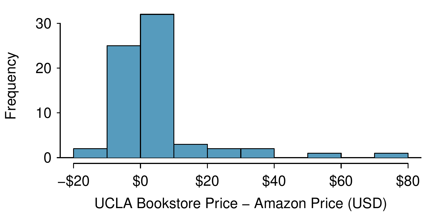
It is important that we always subtract using a consistent order; here Amazon prices are always subtracted from UCLA prices. The first difference shown in Figure 7.2.1 is computed as \(47.97 - 47.45 = 0.52\text{.}\) Similarly, the second difference is computed as \(14.26 - 13.55 = 0.71\text{,}\) and the third is \(13.50 - 12.53 = 0.97\text{.}\) A histogram of the differences is shown in Figure 7.2.2. Using differences between paired observations is a common and useful way to analyze paired data.
Set up a hypothesis test to determine whether, on average, there is a difference between Amazon’s price for a book and the UCLA bookstore’s price. Also, check the conditions for whether we can move forward with the test using the \(t\)-distribution.
Next, we check the independence and normality conditions. The observations are based on a simple random sample, so independence is reasonable. While there are some outliers, \(n = 68\) and none of the outliers are particularly extreme, so the normality of \(\bar{x}\) is satisfied. With these conditions satisfied, we can move forward with the \(t\)-distribution.
To compute the test statistic, we compute the standard error associated with \(\bar{x}_{\text{diff}}\) using the standard deviation of the differences (\(s_{\text{diff}} = 13.42\)) and the number of differences (\(n_{\text{diff}} = 68\)):
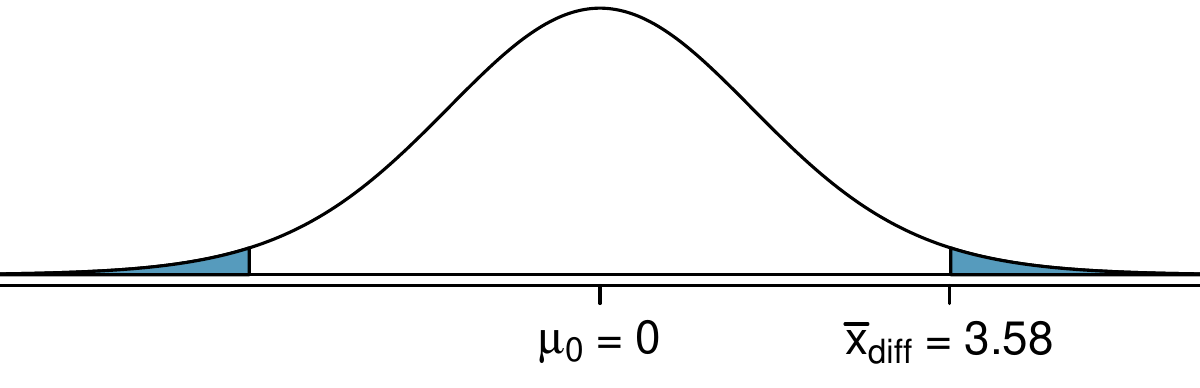
To visualize the p-value, the sampling distribution of \(\bar{x}_{\text{diff}}\) is drawn as though \(H_0\) is true, and the p-value is represented by the two shaded tails:
The degrees of freedom is \(df = 68 - 1 = 67\text{.}\) Using statistical software, we find the one-tail area of 0.0156. Doubling this area gives the p-value: 0.0312.
Because the p-value is less than 0.05, we reject the null hypothesis. Amazon prices are, on average, lower than the UCLA Bookstore prices for UCLA courses.
Create a 95% confidence interval for the average price difference between books at the UCLA bookstore and books on Amazon. 1
Conditions have already been verified and the standard error computed in Example 7.2.4. To find the interval, identify \(t^{\star}_{67}\) using statistical software or the \(t\)-table (\(t^{\star}_{67} = 2.00\)), and plug it, the point estimate, and the standard error into the confidence interval formula: \(\text{point estimate} \pm t^{\star} \times SE \to 3.58 \pm 2.00 \times 1.63 \to (0.32, 6.84)\text{.}\) We are 95% confident that Amazon is, on average, between $0.32 and $6.84 less expensive than the UCLA Bookstore for UCLA course books.
We have strong evidence that Amazon is, on average, less expensive. How should this conclusion affect UCLA student buying habits? Should UCLA students always buy their books on Amazon? 2
The average price difference is only mildly useful for this question. Examine the distribution shown in Figure 7.2.2. There are certainly a handful of cases where Amazon prices are far below the UCLA Bookstore’s, which suggests it is worth checking Amazon (and probably other online sites) before purchasing. However, in many cases the Amazon price is above what the UCLA Bookstore charges, and most of the time the price isn’t that different. Ultimately, if getting a book immediately from the bookstore is notably more convenient, e.g. to get started on reading or homework, it’s likely a good idea to go with the UCLA Bookstore unless the price difference on a specific book happens to be quite large. For reference, this is a very different result from what we (the authors) had seen in a similar data set from 2010. At that time, Amazon prices were almost uniformly lower than those of the UCLA Bookstore’s and by a large margin, making the case to use Amazon over the UCLA Bookstore quite compelling at that time. Now we frequently check multiple websites to find the best price.
Air quality measurements were collected in a random sample of 25 country capitals in 2013, and then again in the same cities in 2014. We would like to use these data to compare average air quality between the two years. Should we use a paired or non-paired test? Explain your reasoning.
Consider two sets of data that are paired with each other. Each observation in one data set has a natural correspondence with exactly one observation from the other data set.
Consider two sets of data that are paired with each other. Each observation in one data set is subtracted from the average of the other data set’s observations.
We would like to know if Intel’s stock and Southwest Airlines’ stock have similar rates of return. To find out, we take a random sample of 50 days, and record Intel’s and Southwest’s stock on those same days.
We randomly sample 50 items from Target stores and note the price for each. Then we visit Walmart and collect the price for each of those same 50 items.
A school board would like to determine whether there is a difference in average SAT scores for students at one high school versus another high school in the district. To check, they take a simple random sample of 100 students from each high school.
Let’s consider a limited set of climate data, examining temperature differences in 1948 vs 2018. We sampled 197 locations from the National Oceanic and Atmospheric Administration’s (NOAA) historical data, where the data was available for both years of interest. We want to know: were there more days with temperatures exceeding 90°F in 2018 or in 1948? The difference in number of days exceeding 90°F (number of days in 2018 - number of days in 1948) was calculated for each of the 197 locations. The average of these differences was 2.9 days with a standard deviation of 17.2 days. We are interested in determining whether these data provide strong evidence that there were more days in 2018 that exceeded 90°F from NOAA’s weather stations.
Based on the results of this hypothesis test, would you expect a confidence interval for the average difference between the number of days exceeding 90°F from 1948 and 2018 to include 0? Explain your reasoning.
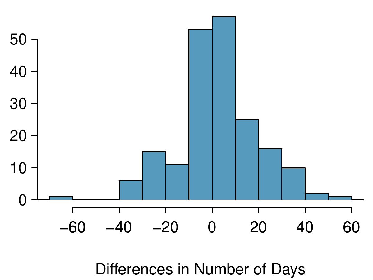
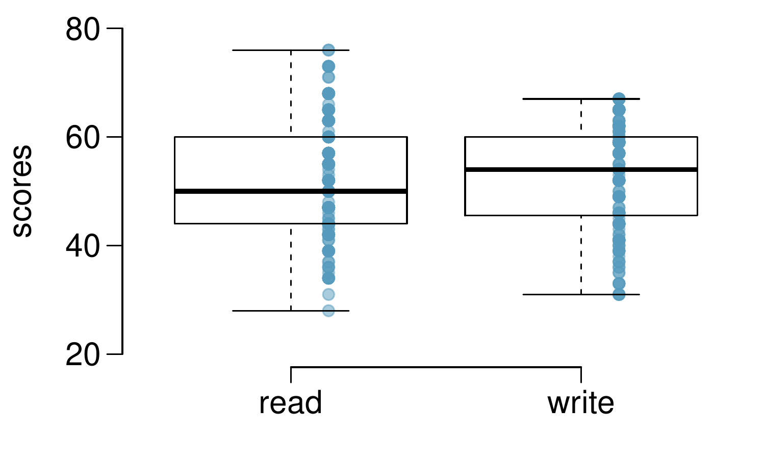
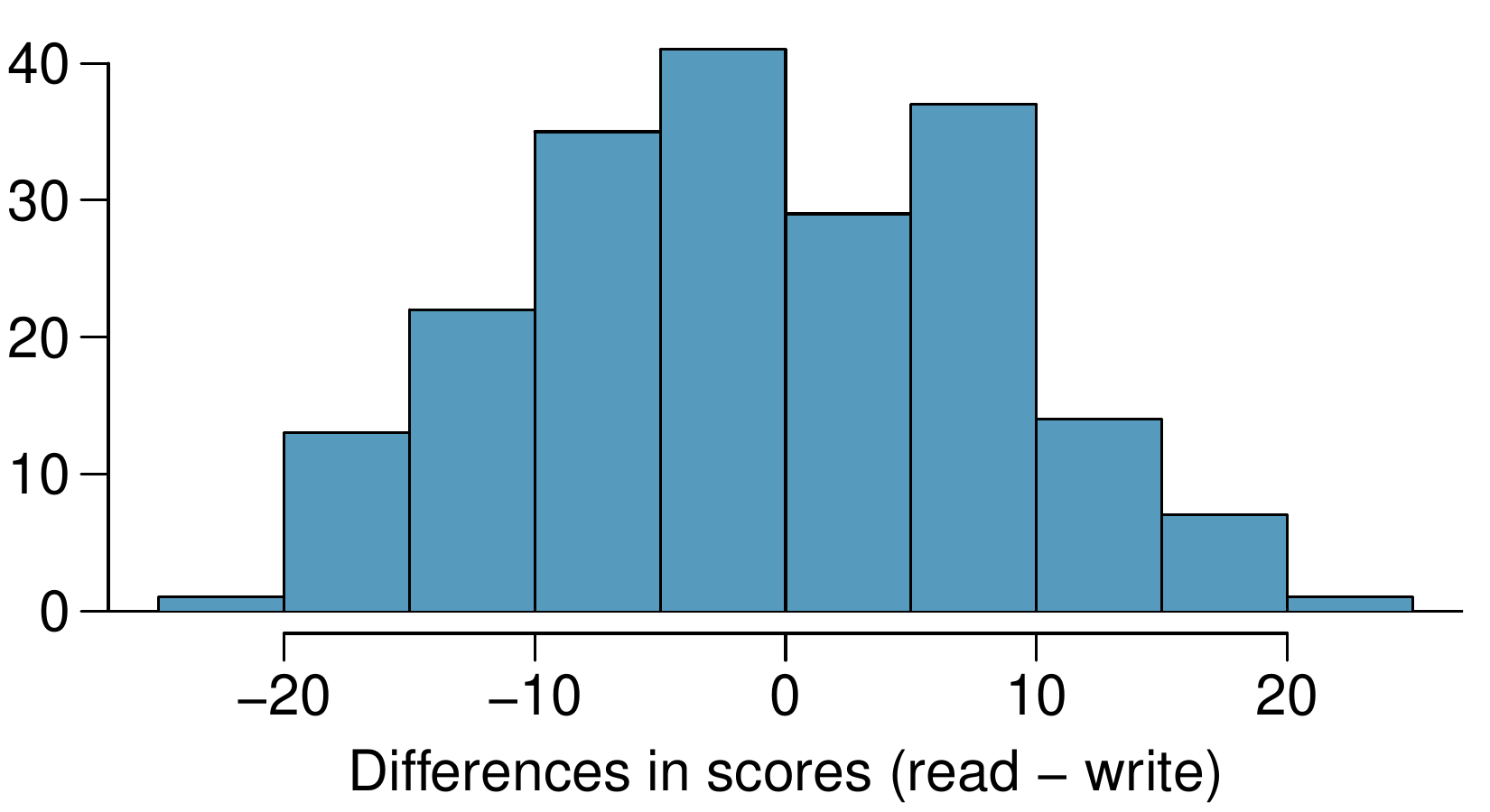
The National Center of Education Statistics conducted a survey of high school seniors, collecting test data on reading, writing, and several other subjects. Here we examine a simple random sample of 200 students from this survey. Side-by-side box plots of reading and writing scores as well as a histogram of the differences in scores are shown below.
Create hypotheses appropriate for the following research question: is there an evident difference in the average scores of students in the reading and writing exam?
The average observed difference in scores is \(\bar{x}_{\text{read-write}} = -0.545\text{,}\) and the standard deviation of the differences is 8.887 points. Do these data provide convincing evidence of a difference between the average scores on the two exams?
Based on the results of this hypothesis test, would you expect a confidence interval for the average difference between the reading and writing scores to include 0? Explain your reasoning.
We considered the change in the number of days exceeding 90°F from 1948 and 2018 at 197 randomly sampled locations from the NOAA database in Exercise 7.2.3.5. The mean and standard deviation of the reported differences are 2.9 days and 17.2 days.
Calculate a 90% confidence interval for the average difference between number of days exceeding 90°F between 1948 and 2018. We’ve already checked the conditions for you.
We considered the differences between the reading and writing scores of a random sample of 200 students who took the High School and Beyond Survey in Exercise 7.2.3.6. The mean and standard deviation of the differences are \(\bar{x}_{\text{read-write}} = -0.545\) and 8.887 points.