Inference for linear regression

Section 8.4 Inference for linear regression

In this section, we discuss uncertainty in the estimates of the slope and y-intercept for a regression line. Just as we identified standard errors for point estimates in previous chapters, we first discuss standard errors for these new estimates.

🔗

Subsection 8.4.1 Midterm elections and unemployment

Elections for members of the United States House of Representatives occur every two years, coinciding every four years with the U.S. Presidential election. The set of House elections occurring during the middle of a Presidential term are called midterm elections. In America’s two-party system, one political theory suggests the higher the unemployment rate, the worse the President’s party will do in the midterm elections.

🔗

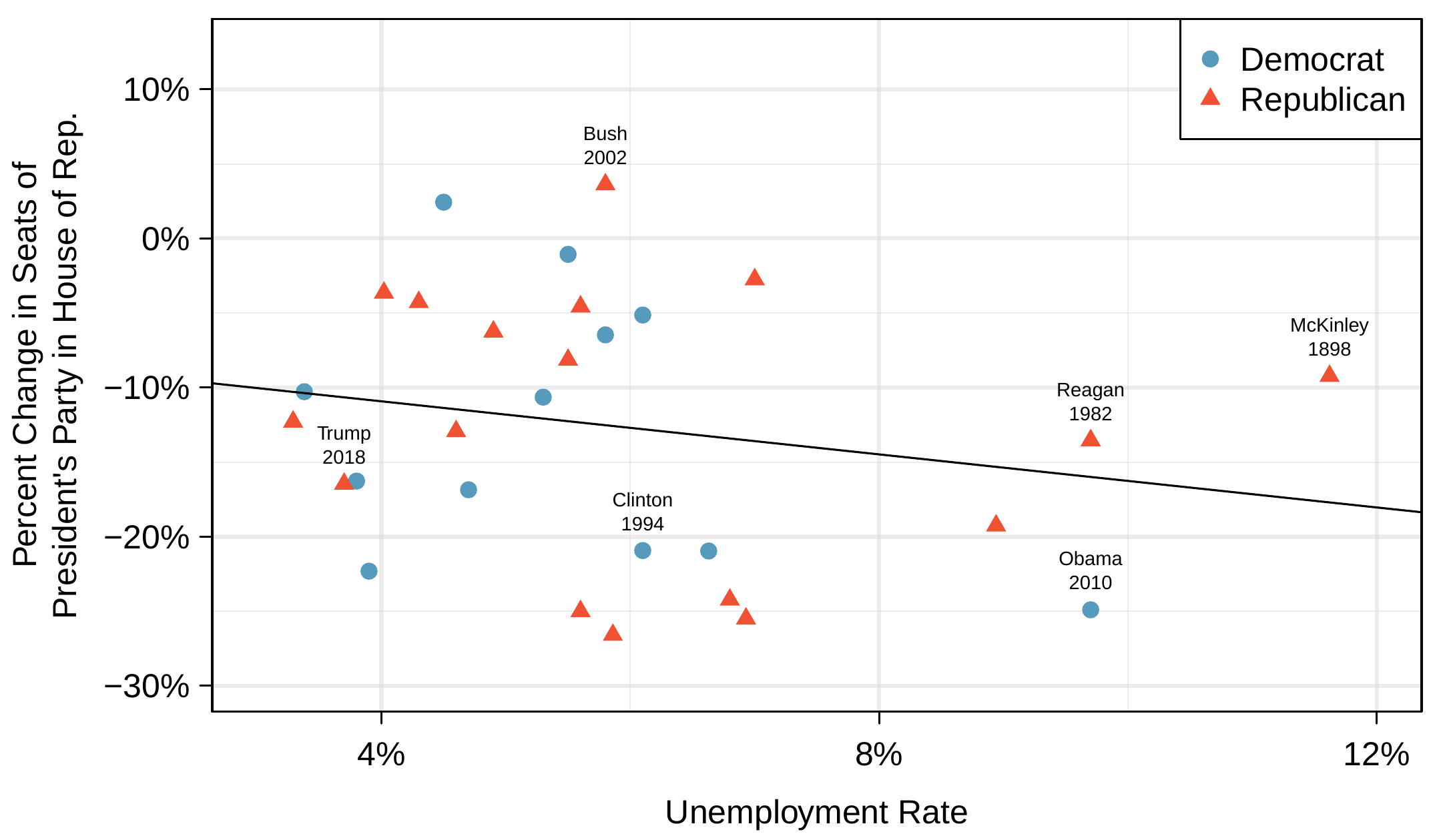
To assess the validity of this claim, we can compile historical data and look for a connection. We consider every midterm election from 1898 to 2018, with the exception of those elections during the Great Depression. Figure 8.4.1 shows these data and the least-squares regression line:

\begin{align*} \amp\text{% change in House seats for President's party}\\ \amp\qquad\qquad= -7.36 - 0.89 \times \text{(unemployment rate)} \end{align*}

We consider the percent change in the number of seats of the President’s party (e.g. percent change in the number of seats for Republicans in 2018) against the unemployment rate.

🔗

Examining the data, there are no clear deviations from linearity, the constant variance condition, or substantial outliers. While the data are collected sequentially, a separate analysis was used to check for any apparent correlation between successive observations; no such correlation was found.

🔗

A scatterplot is shown for the percent change in House seats for the President’s party in each midterm election from 1898 to 2018 plotted against the unemployment rate. The two points for the Great Depression have been removed, and a least squares regression line has been fit to the data with a slightly downward trend. The horizontal axis is for "Unemployment Rate" with values ranging from about 3% to 12%. The vertical axis is for "Percent Change in Seats of the President’s Party in the House of Representatives" with values ranging from about -30% to positive 10%. The bulk of the observations have Unemployment Rate between 3% and 8%, and these have the percent change in seats ranging from about -27% to positive 4% without any discernible trend. There are four observations with unemployment rate above 8%, and these have the percent change in seats ranging from -25% to -9%. Each point in the scatterplot is also labeled as "Democrat" in blue or "Republican" in red, though this doesn’t reveal any additional pattern. — Figure 8.4.1. The percent change in House seats for the President’s party in each midterm election from 1898 to 2018 plotted against the unemployment rate. The two points for the Great Depression have been removed, and a least squares regression line has been fit to the data.
🔗

Checkpoint 8.4.2.

The data for the Great Depression (1934 and 1938) were removed because the unemployment rate was 21% and 18%, respectively. Do you agree that they should be removed for this investigation? Why or why not?

🔗

Solution.

We will provide two considerations. Each of these points would have very high leverage on any least-squares regression line, and years with such high unemployment may not help us understand what would happen in other years where the unemployment is only modestly high. On the other hand, these are exceptional cases, and we would be discarding important information if we exclude them from a final analysis.

🔗

There is a negative slope in the line shown in Figure 8.4.1. However, this slope (and the y-intercept) are only estimates of the parameter values. We might wonder, is this convincing evidence that the “true” linear model has a negative slope? That is, do the data provide strong evidence that the political theory is accurate, where the unemployment rate is a useful predictor of the midterm election? We can frame this investigation into a statistical hypothesis test:

$H_0\text{:}$ $\beta_1 = 0\text{.}$ The true linear model has slope zero.

🔗
$H_A\text{:}$ $\beta_1 \neq 0\text{.}$ The true linear model has a slope different than zero. The unemployment is predictive of whether the President’s party wins or loses seats in the House of Representatives.

🔗

We would reject $H_0$ in favor of $H_A$ if the data provide strong evidence that the true slope parameter is different than zero. To assess the hypotheses, we identify a standard error for the estimate, compute an appropriate test statistic, and identify the p-value.

🔗

Subsection 8.4.2 Understanding regression output from software

Just like other point estimates we have seen before, we can compute a standard error and test statistic for $b_1\text{.}$ We will generally label the test statistic using a $T\text{,}$ since it follows the $t$-distribution.

🔗

We will rely on statistical software to compute the standard error and leave the explanation of how this standard error is determined to a second or third statistics course. Figure 8.4.3 shows software output for the least squares regression line in Figure 8.4.1. The row labeled unemp includes the point estimate and other hypothesis test information for the slope, which is the coefficient of the unemployment variable.

🔗

	Estimate	Std. Error	t value	Pr($>$\|t\|)
(Intercept)	-7.3644	5.1553	-1.43	0.1646
unemp	-0.8897	0.8350	-1.07	0.2961
$df=27$

Figure 8.4.3. Output from statistical software for the regression line modeling the midterm election losses for the President’s party as a response to unemployment.

🔗

Example 8.4.4.

What do the first and second columns of Figure 8.4.3 represent?

🔗

Solution.

The entries in the first column represent the least squares estimates, $b_0$ and $b_1\text{,}$ and the values in the second column correspond to the standard errors of each estimate. Using the estimates, we could write the equation for the least square regression line as

\begin{equation*} \hat{y} = -7.3644 - 0.8897 x \end{equation*}

where $\hat{y}$ in this case represents the predicted change in the number of seats for the president’s party, and $x$ represents the unemployment rate.

🔗

We previously used a $t$-test statistic for hypothesis testing in the context of numerical data. Regression is very similar. In the hypotheses we consider, the null value for the slope is 0, so we can compute the test statistic using the T (or Z) score formula:

\begin{equation*} T = \frac{\text{estimate} - \text{null value}}{\text{SE}} = \frac{-0.8897 - 0}{0.8350} = -1.07 \end{equation*}

This corresponds to the third column of Figure 8.4.3.

🔗

Example 8.4.5.

Use the table in Figure 8.4.3 to determine the p-value for the hypothesis test.

🔗

Solution.

The last column of the table gives the p-value for the two-sided hypothesis test for the coefficient of the unemployment rate: 0.2961. That is, the data do not provide convincing evidence that a higher unemployment rate has any correspondence with smaller or larger losses for the President’s party in the House of Representatives in midterm elections.

🔗

Inference for regression.

We usually rely on statistical software to identify point estimates, standard errors, test statistics, and p-values in practice. However, be aware that software will not generally check whether the method is appropriate, meaning we must still verify conditions are met.

🔗

Example 8.4.6.

Examine Figure 8.2.13, which relates the Elmhurst College aid and student family income. How sure are you that the slope is statistically significantly different from zero? That is, do you think a formal hypothesis test would reject the claim that the true slope of the line should be zero?

🔗

Solution.

While the relationship between the variables is not perfect, there is an evident decreasing trend in the data. This suggests the hypothesis test will reject the null claim that the slope is zero.

🔗

Checkpoint 8.4.7.

Figure 8.4.8 shows statistical software output from fitting the least squares regression line shown in Figure 8.2.13. Use this output to formally evaluate the following hypotheses.

$H_0\text{:}$ The true coefficient for family income is zero.

🔗
$H_A\text{:}$ The true coefficient for family income is not zero.

🔗

🔗

Solution.

We look in the second row corresponding to the family income variable. We see the point estimate of the slope of the line is -0.0431, the standard error of this estimate is 0.0108, and the $t$-test statistic is $T = -3.98\text{.}$ The p-value corresponds exactly to the two-sided test we are interested in: 0.0002. The p-value is so small that we reject the null hypothesis and conclude that family income and financial aid at Elmhurst College for freshman entering in the year 2011 are negatively correlated and the true slope parameter is indeed less than 0, just as we believed in Example 8.4.6.

🔗

	Estimate	Std. Error	t value	Pr($>$\|t\|)
(Intercept)	24319.3	1291.5	18.83	$\lt$0.0001
family_income	-0.0431	0.0108	-3.98	0.0002
$df=48$

Figure 8.4.8. Summary of least squares fit for the Elmhurst College data, where we are predicting the gift aid by the university based on the family income of students.

🔗

Subsection 8.4.3 Confidence interval for a coefficient

Similar to how we can conduct a hypothesis test for a model coefficient using regression output, we can also construct a confidence interval for that coefficient.

🔗

Example 8.4.9.

Compute the 95% confidence interval for the family_income coefficient using the regression output from Figure 8.4.8.

🔗

Solution.

The point estimate is -0.0431 and the standard error is $SE = 0.0108\text{.}$ When constructing a confidence interval for a model coefficient, we generally use a $t$-distribution. The degrees of freedom for the distribution are noted in the regression output, $df = 48\text{,}$ allowing us to identify $t_{48}^{\star} = 2.01$ for use in the confidence interval.

🔗

We can now construct the confidence interval in the usual way:

\begin{align*} \text{point estimate} \pm t_{48}^{\star} \times SE \amp\to -0.0431 \pm 2.01 \times 0.0108\\ \amp\to (-0.0648, -0.0214) \end{align*}

We are 95% confident that with each dollar increase in family_income, the university’s gift aid is predicted to decrease on average by $0.0214 to $0.0648.

🔗

Confidence intervals for coefficients.

Confidence intervals for model coefficients can be computed using the $t$-distribution:

\begin{equation*} b_i \ \pm\ t_{df}^{\star} \times SE_{b_{i}} \end{equation*}

where $t_{df}^{\star}$ is the appropriate $t$-value corresponding to the confidence level with the model’s degrees of freedom.

🔗

On the topic of intervals in this book, we’ve focused exclusively on confidence intervals for model parameters. However, there are other types of intervals that may be of interest, including prediction intervals for a response value and also confidence intervals for a mean response value in the context of regression. These two interval types are introduced in an online extra supplied by OpenIntro that you may download at www.openintro.org/d?file=stat_extra_linear_regression_supp

🔗

Exercises 8.4.4 Section Exercises

In the following exercises, visually check the conditions for fitting a least squares regression line. However, you do not need to report these conditions in your solutions.

🔗

1. Body measurements, Part IV.

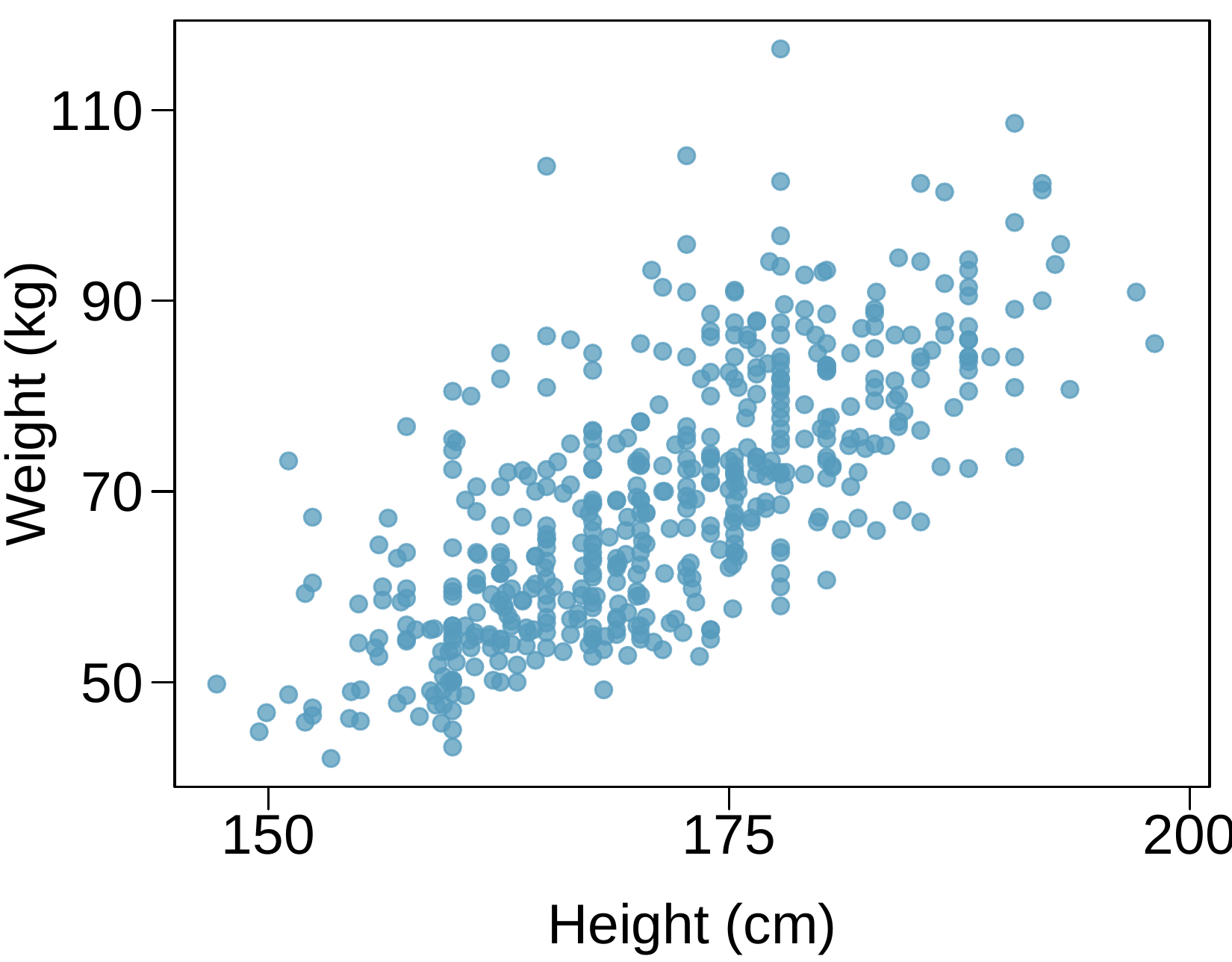
The scatterplot and least squares summary below show the relationship between weight measured in kilograms and height measured in centimeters of 507 physically active individuals.

🔗

A scatterplot is shown with around 500 points. The horizontal axis is for "Height, in centimeters" and takes values between about 150 to 200 centimeters. The vertical axis is for "Weight, in kilograms" and takes values between about 40 to 120 kilograms. For heights smaller than about 160 centimeters, weights mostly range between 45 and 70 kilograms. For heights between 160 and 175 centimeters, weights mostly range between 55 and 80 kilograms. For heights between 175 and 185 centimeters, weights mostly range between 65 and 90 kilograms. For heights between 185 and 195 centimeters, where there are fewer points, weights mostly range between 80 and 95 kilograms. There are two points with heights at about 196cm, and these have weights of about 85 and 95 kilograms.

	Estimate	Std. Error	t value	Pr($>$\|t\|)
(Intercept)	-105.0113	7.5394	-13.93	0.0000
height	1.0176	0.0440	23.13	0.0000

Describe the relationship between height and weight.

🔗
Write the equation of the regression line. Interpret the slope and intercept in context.

🔗
Do the data provide strong evidence that an increase in height is associated with an increase in weight? State the null and alternative hypotheses, report the p-value, and state your conclusion.

🔗
The correlation coefficient for height and weight is 0.72. Calculate $R^2$ and interpret it in context.

🔗

🔗

2. Beer and blood alcohol content.

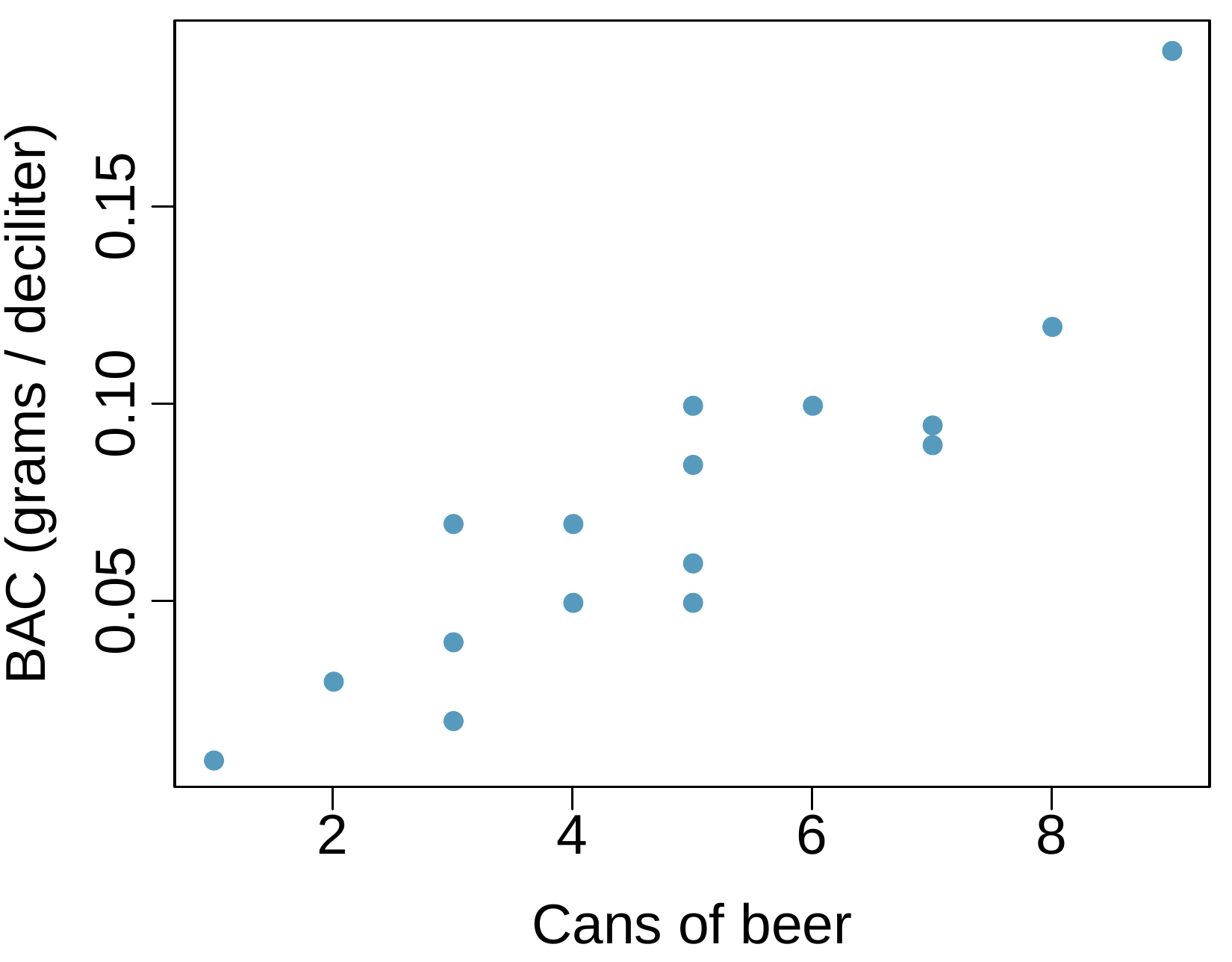
Many people believe that gender, weight, drinking habits, and many other factors are much more important in predicting blood alcohol content (BAC) than simply considering the number of drinks a person consumed. Here we examine data from sixteen student volunteers at Ohio State University who each drank a randomly assigned number of cans of beer. These students were evenly divided between men and women, and they differed in weight and drinking habits. Thirty minutes later, a police officer measured their blood alcohol content (BAC) in grams of alcohol per deciliter of blood. The scatterplot and regression table summarize the findings.

🔗

A scatterplot is shown with around 15 points. The horizontal axis is for "Cans of beer" and takes values between about 1 and 9. The vertical axis is for "Blood Alcohol Concentration (BAC), in grams per deciliter" and takes values between about 0.01 to 0.2. The point at 1 can of beer is at 0.01 BAC, lower than any other values. For the four points at 2 and 3 cans of beer, BAC ranges from 0.02 to 0.07. For the six points at 4 and 5 cans of beer, BAC ranges from 0.05 to 0.10. Two points are at 7 cans of beer and have BAC of 0.09 and 0.10. There is a single point for 8 cans of beer, which has a BAC of 0.12, and one last point at 9 cans of beer, which has a BAC of about 0.19.

	Estimate	Std. Error	t value	Pr($>$\|t\|)
(Intercept)	-0.0127	0.0126	-1.00	0.3320
beers	0.0180	0.0024	7.48	0.0000

Describe the relationship between the number of cans of beer and BAC.

🔗
Write the equation of the regression line. Interpret the slope and intercept in context.

🔗
Do the data provide strong evidence that drinking more cans of beer is associated with an increase in blood alcohol? State the null and alternative hypotheses, report the p-value, and state your conclusion.

🔗
The correlation coefficient for number of cans of beer and BAC is 0.89. Calculate $R^2$ and interpret it in context.

🔗
Suppose we visit a bar, ask people how many drinks they have had, and also take their BAC. Do you think the relationship between number of drinks and BAC would be as strong as the relationship found in the Ohio State study?

🔗

🔗

3. Husbands and wives, Part II.

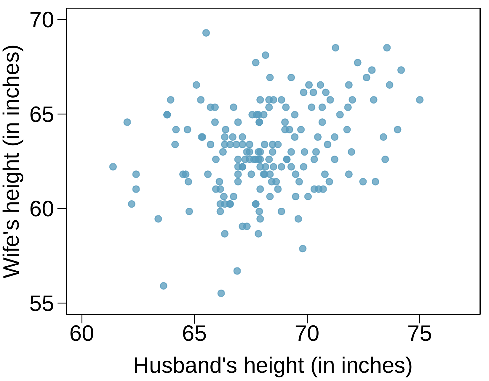
The scatterplot below summarizes husbands’ and wives’ heights in a random sample of 170 married couples in Britain, where both partners’ ages are below 65 years. Summary output of the least squares fit for predicting wife’s height from husband’s height is also provided in the table.

🔗

A scatterplot is shown with around 200 points. The horizontal axis is for "Husband’s height, in inches" and takes values between 60 and 75 inches. The vertical axis is for "Wife’s height, in inches" and takes values between 55 and 70 inches. For the approximately fifteen husband heights smaller than 65 inches, wife heights are mostly between 59 and 65 inches. For the approximately 100 husband heights between 65 and 70 inches, wife heights are mostly between 59 and 66 inches. For the approximately 30 husband heights taller than 70 inches, wife heights are mostly between 62 and 67 inches.

	Estimate	Std. Error	t value	Pr($>$\|t\|)
(Intercept)	43.5755	4.6842	9.30	0.0000
height_husband	0.2863	0.0686	4.17	0.0000

Is there strong evidence that taller men marry taller women? State the hypotheses and include any information used to conduct the test.

🔗
Write the equation of the regression line for predicting wife’s height from husband’s height.

🔗
Interpret the slope and intercept in the context of the application.

🔗
Given that $R^2 = 0.09\text{,}$ what is the correlation of heights in this data set?

🔗
You meet a married man from Britain who is 5’9" (69 inches). What would you predict his wife’s height to be? How reliable is this prediction?

🔗
You meet another married man from Britain who is 6’7" (79 inches). Would it be wise to use the same linear model to predict his wife’s height? Why or why not?

🔗

🔗

4. Urban homeowners, Part II.

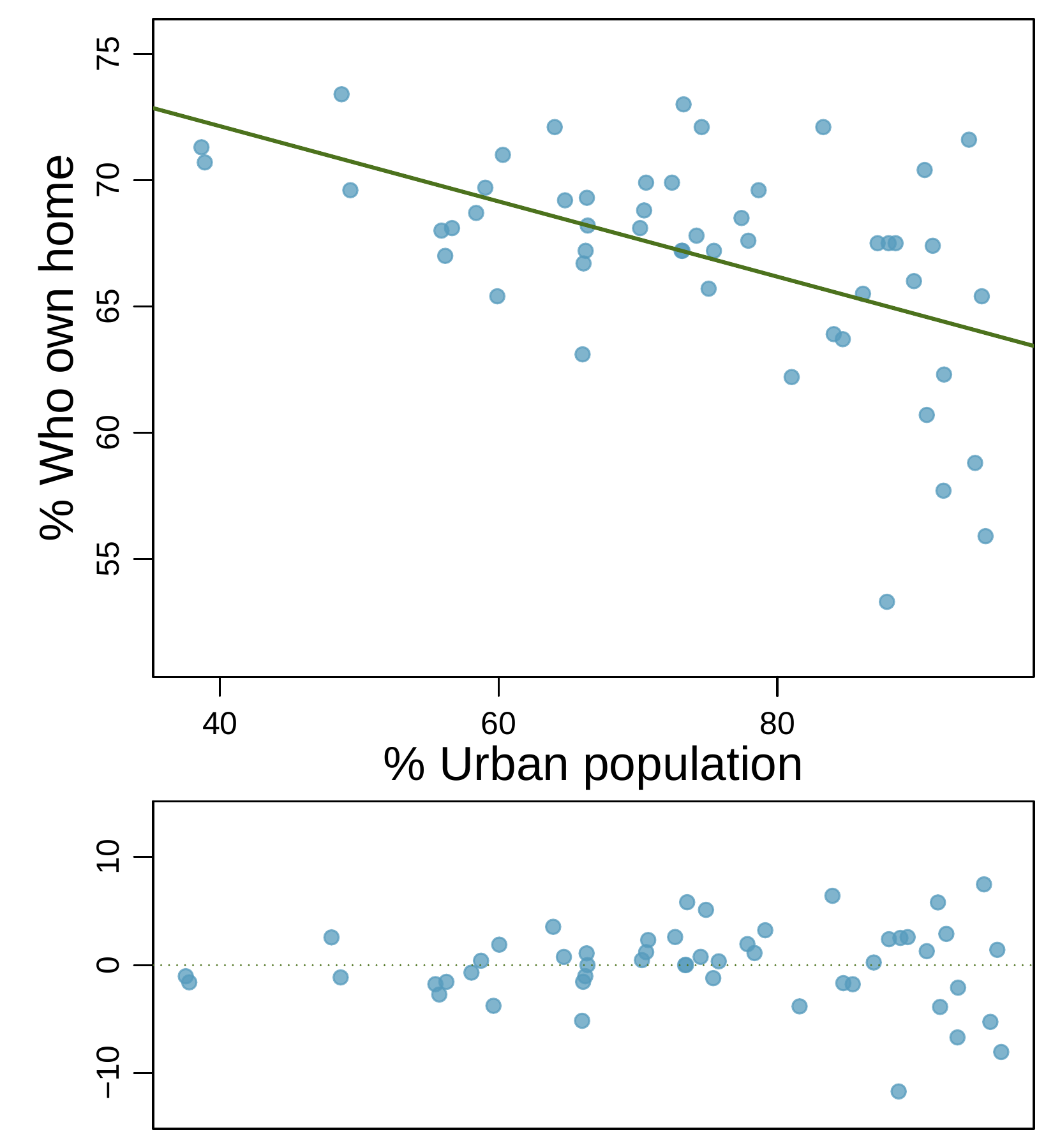
Exercise 8.3.3 gives a scatterplot displaying the relationship between the percent of families that own their home and the percent of the population living in urban areas. Below is a similar scatterplot, excluding District of Columbia, as well as the residuals plot. There were 51 cases.

🔗

A scatterplot showing the relationship between percent of the population living in urban areas (horizontal axis) and the percent of families that own their home (vertical axis), excluding District of Columbia. The scatterplot shows data points scattered with an apparent trend, along with a corresponding residual plot to assess the fit of a linear model. — Figure 8.4.10.
🔗

For these data, $R^2=0.28\text{.}$ What is the correlation? How can you tell if it is positive or negative?

🔗
Examine the residual plot. What do you observe? Is a simple least squares fit appropriate for these data?

🔗

🔗

5. Murders and poverty, Part II.

Exercise 8.2.9.9 presents regression output from a model for predicting annual murders per million from percentage living in poverty based on a random sample of 20 metropolitan areas. The model output is also provided below.

🔗

	Estimate	Std. Error	t value	Pr($>$\|t\|)
(Intercept)	-29.901	7.789	-3.839	0.001
poverty%	2.559	0.390	6.562	0.000

$s = 5.512$ $\qquad$ $R^2 = 70.52\%$ $\qquad$ $R^2_{adj} = 68.89\%$

🔗

What are the hypotheses for evaluating whether poverty percentage is a significant predictor of murder rate?

🔗
State the conclusion of the hypothesis test from part (a) in context of the data.

🔗
Calculate a 95% confidence interval for the slope of poverty percentage, and interpret it in context of the data.

🔗
Do your results from the hypothesis test and the confidence interval agree? Explain.

🔗

🔗

6. Babies.

Is the gestational age (time between conception and birth) of a low birth-weight baby useful in predicting head circumference at birth? Twenty-five low birth-weight babies were studied at a Harvard teaching hospital; the investigators calculated the regression of head circumference (measured in centimeters) against gestational age (measured in weeks). The estimated regression line is

\begin{equation*} \widehat{\text{head circumference}} = 3.91 + 0.78 \times \text{gestational age} \end{equation*}

🔗

What is the predicted head circumference for a baby whose gestational age is 28 weeks?

🔗
The standard error for the coefficient of gestational age is 0.35, which is associated with $df=23\text{.}$ Does the model provide strong evidence that gestational age is significantly associated with head circumference?

🔗

🔗

Prev Top Next