Continuous distributions

Section 3.5 Continuous distributions

So far in this chapter we’ve discussed cases where the outcome of a variable is discrete. In this section, we consider a context where the outcome is a continuous numerical variable.

🔗

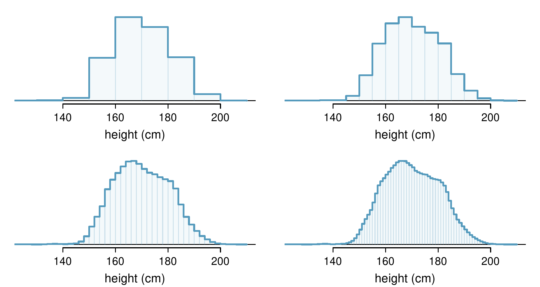
Example 3.5.1. US adult heights histograms.

Figure 3.5.2 shows a few different hollow histograms for the heights of US adults. How does changing the number of bins allow you to make different interpretations of the data?

🔗

Solution.

Adding more bins provides greater detail. This sample is extremely large, which is why much smaller bins still work well. Usually we do not use so many bins with smaller sample sizes since small counts per bin mean the bin heights are very volatile.

🔗

Figure 3.5.2. Four hollow histograms of US adults heights with varying bin widths
🔗

Example 3.5.3. Probability from histogram.

What proportion of the sample is between 180 cm and 185 cm tall (about 5’11" to 6’1")?

🔗

Solution.

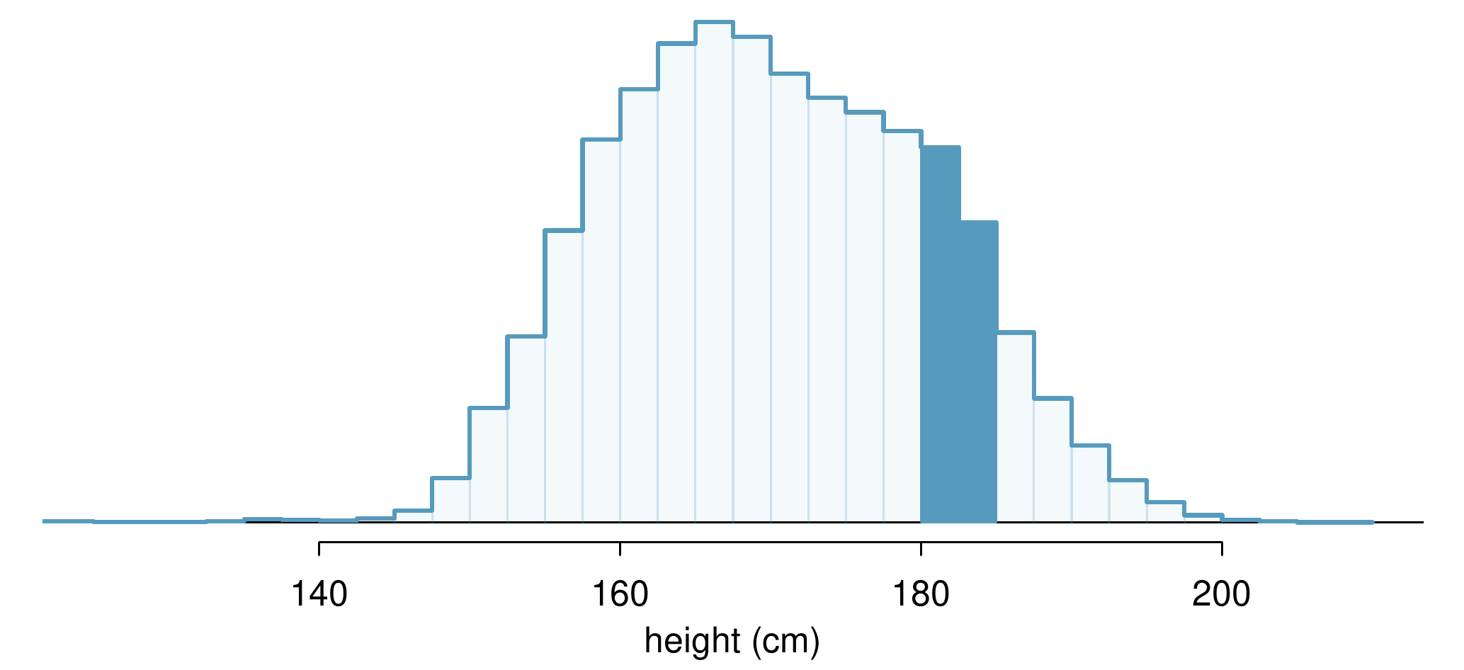
We can add up the heights of the bins in the range 180 cm and 185 cm and divide by the sample size. For instance, this can be done with the two shaded bins shown in Figure 3.5.4. The two bins in this region have counts of 195,307 and 156,239 people, resulting in the following estimate of the probability:

\begin{equation*} \frac{195307 + 156239}{3,000,000} = 0.1172 \end{equation*}

This fraction is the same as the proportion of the histogram’s area that falls in the range 180 to 185 cm.

🔗

Figure 3.5.4. A histogram with bin sizes of 2.5 cm. The shaded region represents individuals with heights between 180 and 185 cm.
🔗

Subsection 3.5.1 From histograms to continuous distributions

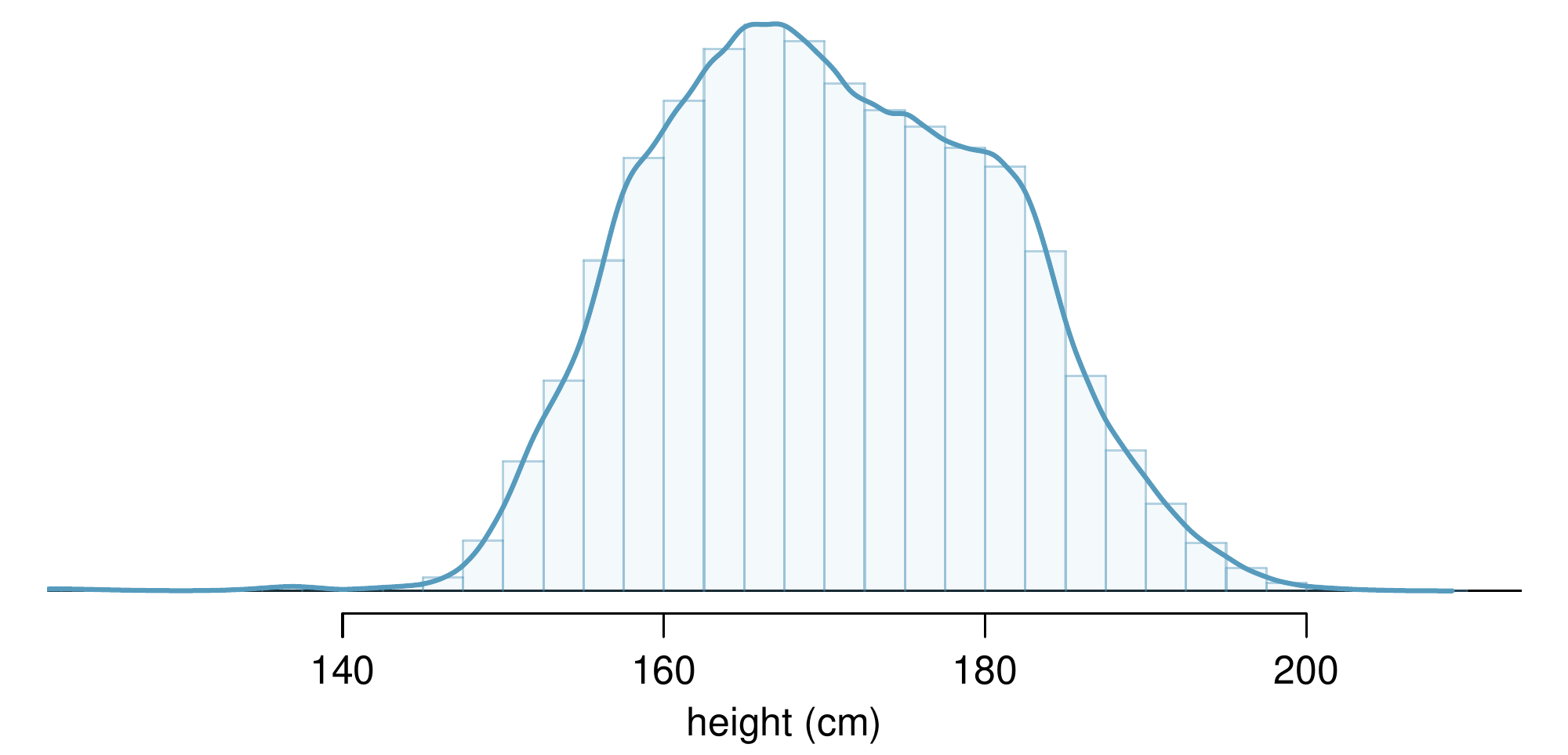
Examine the transition from a boxy hollow histogram in the top-left of Figure 3.5.2 to the much smoother plot in the lower-right. In this last plot, the bins are so slim that the hollow histogram is starting to resemble a smooth curve. This suggests the population height as a continuous numerical variable might best be explained by a curve that represents the outline of extremely slim bins.

🔗

This smooth curve represents a probability density function (also called a density or distribution), and such a curve is shown in Figure 3.5.5 overlaid on a histogram of the sample. A density has a special property: the total area under the density’s curve is 1.

🔗

Figure 3.5.5. The continuous probability distribution of heights for US adults.
🔗

🔗

Subsection 3.5.2 Probabilities from continuous distributions

We computed the proportion of individuals with heights 180 to 185 cm in Example 3.5.3 as a fraction:

\begin{equation*} \frac{\text{number of people between 180 and 185}}{\text{total sample size}} \end{equation*}

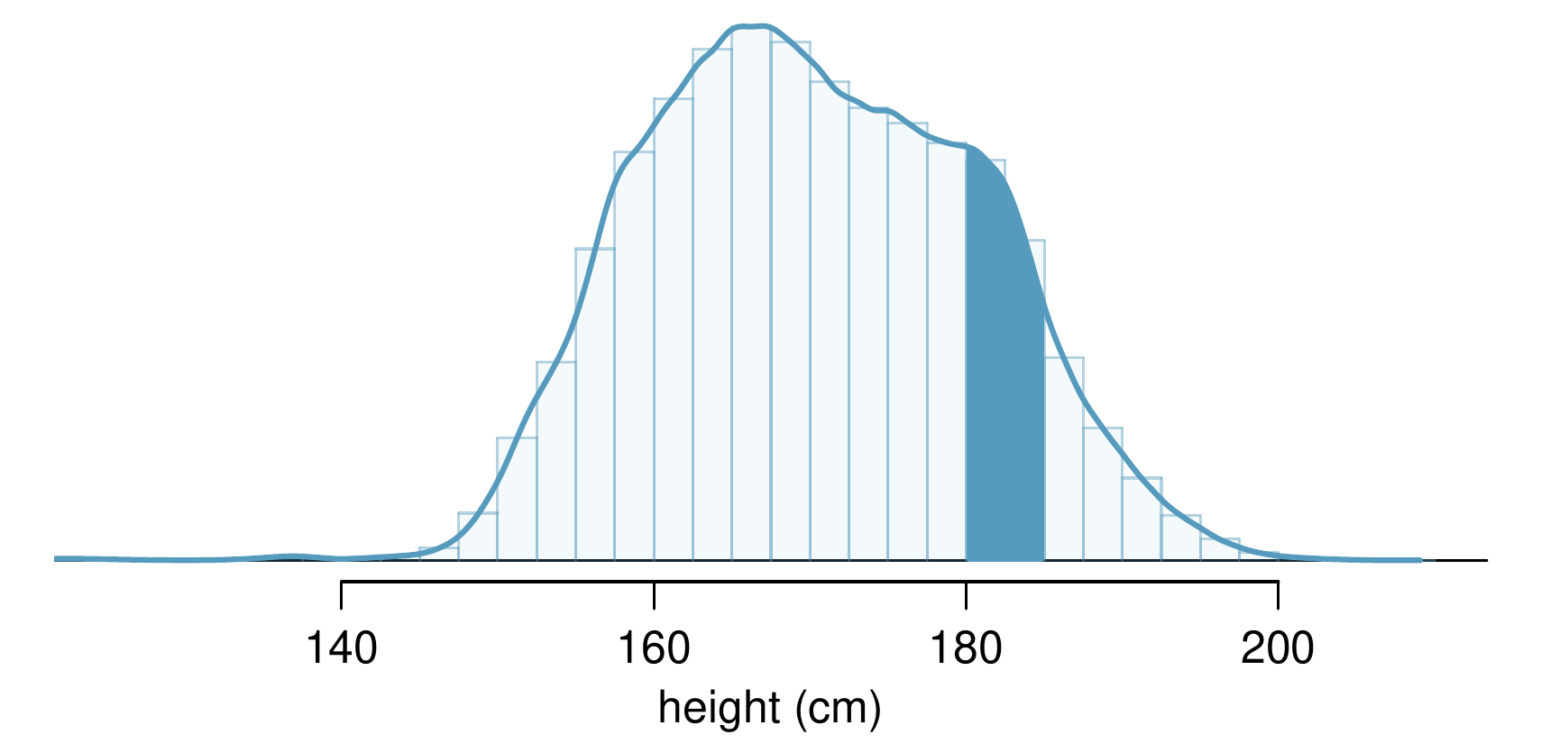
We found the number of people with heights between 180 and 185 cm by determining the fraction of the histogram’s area in this region. Similarly, we can use the area in the shaded region under the curve to find a probability (with the help of a computer):

\begin{equation*} P(\text{height between 180 and 185}) = \text{area between 180 and 185} = 0.1157 \end{equation*}

The probability that a randomly selected person is between 180 and 185 cm is 0.1157. This is very close to the estimate from Example 3.5.3: 0.1172.

🔗

Figure 3.5.6. Density for heights in the US adult population with the area between 180 and 185 cm shaded. Compare this plot with Figure 3.5.4.
🔗

Checkpoint 3.5.7.

Three US adults are randomly selected. The probability a single adult is between 180 and 185 cm is 0.1157.

🔗

What is the probability that all three are between 180 and 185 cm tall?
🔗

🔗
What is the probability that none are between 180 and 185 cm?
🔗

🔗

🔗

Solution.

Brief answers:

$\displaystyle 0.1157 \times 0.1157 \times 0.1157 = 0.0015$
🔗

🔗
$\displaystyle (1 - 0.1157)^3 = 0.692$
🔗

🔗

🔗

Example 3.5.8.

What is the probability that a randomly selected person is exactly 180 cm? Assume you can measure perfectly.

🔗

Solution.

This probability is zero. A person might be close to 180 cm, but not exactly 180 cm tall. This also makes sense with the definition of probability as area; there is no area captured between 180 cm and 180 cm.

🔗

Checkpoint 3.5.9.

Suppose a person’s height is rounded to the nearest centimeter. Is there a chance that a random person’s measured height will be 180 cm?

🔗

Solution.

This has positive probability. Anyone between 179.5 cm and 180.5 cm will have a measured height of 180 cm. This is probably a more realistic scenario to encounter in practice versus Example 3.5.8.

🔗

Exercises 3.5.3 Exercises

1. Cat weights.

The histogram shown below represents the weights (in kg) of 47 female and 97 male cats.

🔗

Figure 3.5.10. Histogram of cat weights
🔗

What fraction of these cats weigh less than 2.5 kg?
🔗

🔗
What fraction of these cats weigh between 2.5 and 2.75 kg?
🔗

🔗
What fraction of these cats weigh between 2.75 and 3.5 kg?
🔗

🔗

🔗

2. Income and gender.

The relative frequency table below displays the distribution of annual total personal income (in 2009 inflation-adjusted dollars) for a representative sample of 96,420,486 Americans. These data come from the American Community Survey for 2005-2009. This sample is comprised of 59% males and 41% females.

🔗

Table 3.5.11. Annual personal income distribution

🔗

Income	Total
$1 to $9,999 or loss	2.2%
$10,000 to $14,999	4.7%
$15,000 to $24,999	15.8%
$25,000 to $34,999	18.3%
$35,000 to $49,999	21.2%
$50,000 to $64,999	13.9%
$65,000 to $74,999	5.8%
$75,000 to $99,999	8.4%
$100,000 or more	9.7%

Describe the distribution of total personal income.
🔗

🔗
What is the probability that a randomly chosen US resident makes less than $50,000 per year?
🔗

🔗
What is the probability that a randomly chosen US resident makes less than $50,000 per year and is female? Note any assumptions you make.
🔗

🔗
The same data source indicates that 71.8% of females make less than $50,000 per year. Use this value to determine whether or not the assumption you made in part (c) is valid.
🔗

🔗

🔗

Prev Top Next