Section 3.4 Random variables

It’s often useful to model a process using what’s called a random variable. Such a model allows us to apply a mathematical framework and statistical principles for better understanding and predicting outcomes in the real world.

Example 3.4.1. Bookstore sales expectation.

Two books are assigned for a statistics class: a textbook and its corresponding study guide. The university bookstore determined 20% of enrolled students do not buy either book, 55% buy the textbook only, and 25% buy both books. If there are 100 students enrolled, how many books should the bookstore expect to sell to this class?

Solution.

Around 20 students will not buy either book (0 books total), about 55 will buy one book (55 books total), and approximately 25 will buy two books (totaling 50 books for these 25 students). The bookstore should expect to sell about 105 books for this class.

Checkpoint 3.4.2.

Would you be surprised if the bookstore sold slightly more or less than 105 books?

Solution.

If they sell a little more or a little less, this should not be a surprise. There is natural variability in observed data. For example, if we flip a coin 100 times, it will not usually come up heads exactly half the time, but it will probably be close.

Subsection 3.4.1 Expectation

We call a variable or process with a numerical outcome a random variable, and we usually represent this random variable with a capital letter such as $X\text{,}$ $Y\text{,}$ or $Z\text{.}$ The amount of money a single student will spend on her statistics books is a random variable, and we represent it by $X\text{.}$

Random variable.

A random process or variable with a numerical outcome.

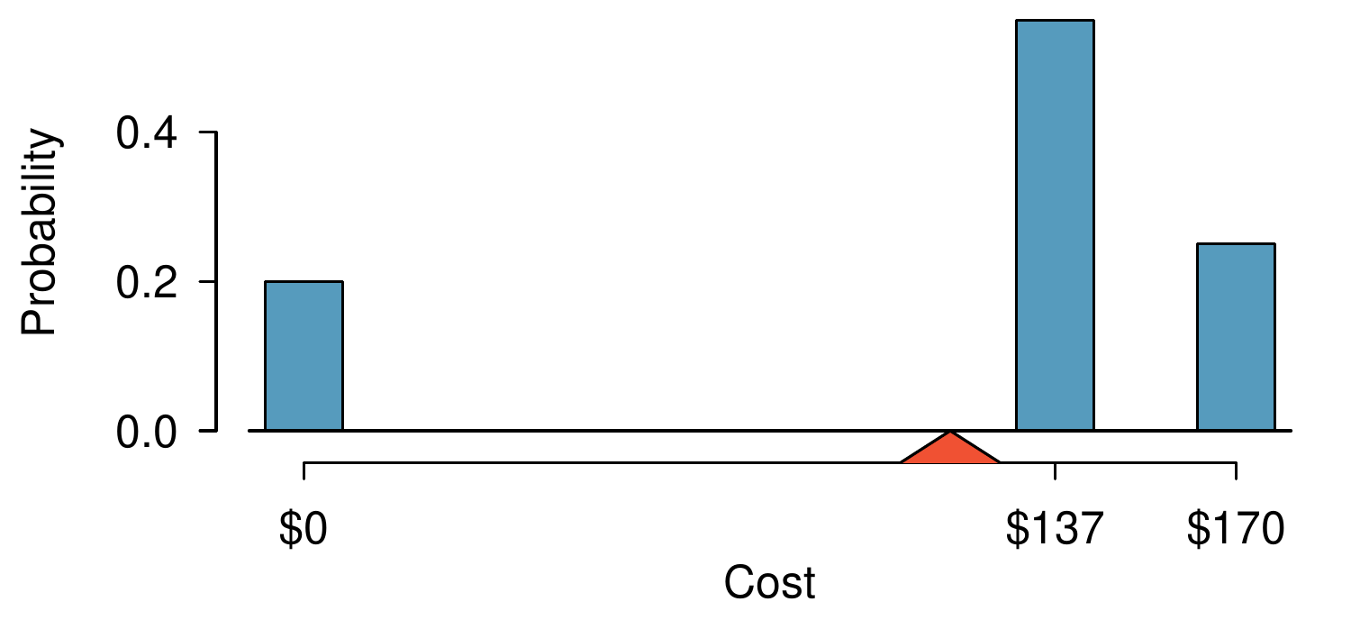
The possible outcomes of $X$ are labeled with a corresponding lower case letter $x$ and subscripts. For example, we write $x_1 = \$0\text{,}$ $x_2 = \$137\text{,}$ and $x_3 = \$170\text{,}$ which occur with probabilities 0.20, 0.55, and 0.25. The distribution of $X$ is summarized in the table below.

$i$	1	2	3	Total
$x_i$	$0	$137	$170	--
$P(X=x_i)$	0.20	0.55	0.25	1.00

Figure 3.4.3. The probability distribution for the random variable $X\text{,}$ representing the bookstore’s revenue from a single student.

Figure 3.4.4. Probability distribution for the bookstore’s revenue from one student. The triangle represents the average revenue per student.

Example 3.4.5.

What is the average revenue per student for this course?

Solution.

The expected total revenue is $11,785, and there are 100 students. Therefore the expected revenue per student is $\$11,785/100 = \$117.85\text{.}$

We computed the average outcome of $X$ as $\$117.85$ in Example 3.4.5. We call this average the expected value of $X\text{,}$ denoted by $E(X)\text{.}$ The expected value of a random variable is computed by adding each outcome weighted by its probability:

\begin{align*} E(X) \amp= 0 \times P(X=0) + 137 \times P(X=137) + 170 \times P(X=170)\\ \amp= 0 \times 0.20 + 137 \times 0.55 + 170 \times 0.25 = 117.85 \end{align*}

Expected value of a discrete random variable.

If $X$ takes outcomes $x_1, \ldots, x_k$ with probabilities $P(X=x_1), \ldots, P(X=x_k)\text{,}$ the expected value of $X$ is the sum of each outcome multiplied by its corresponding probability:

\begin{align*} E(X) \amp= x_1 \times P(X = x_1) + \cdots + x_k \times P(X = x_k)\\ \amp= \sum_{i=1}^{k} x_i P(X = x_i) \end{align*}

The Greek letter $\mu$ may be used in place of the notation $E(X)\text{.}$

The expected value for a random variable represents the average outcome. For example, $E(X) = 117.85$ represents the average amount the bookstore expects to make from a single student, which we could also write as $\mu = 117.85\text{.}$

It is also possible to compute the expected value of a continuous random variable (see Section 3.5). However, it requires calculus and we save it for a later class.

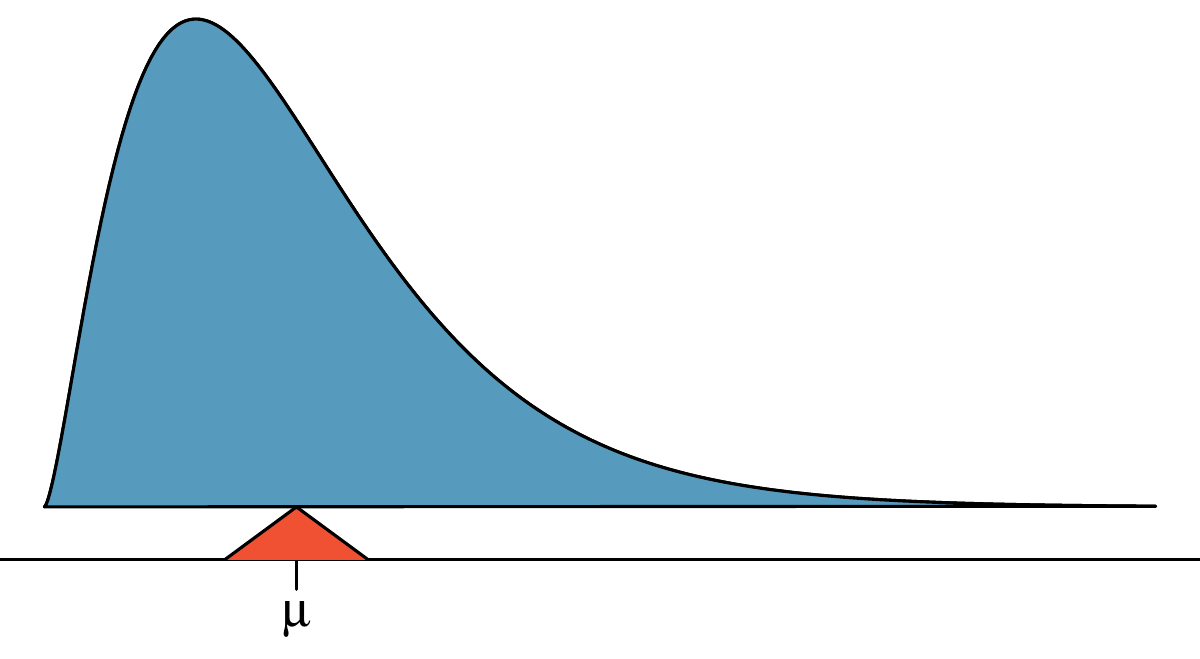
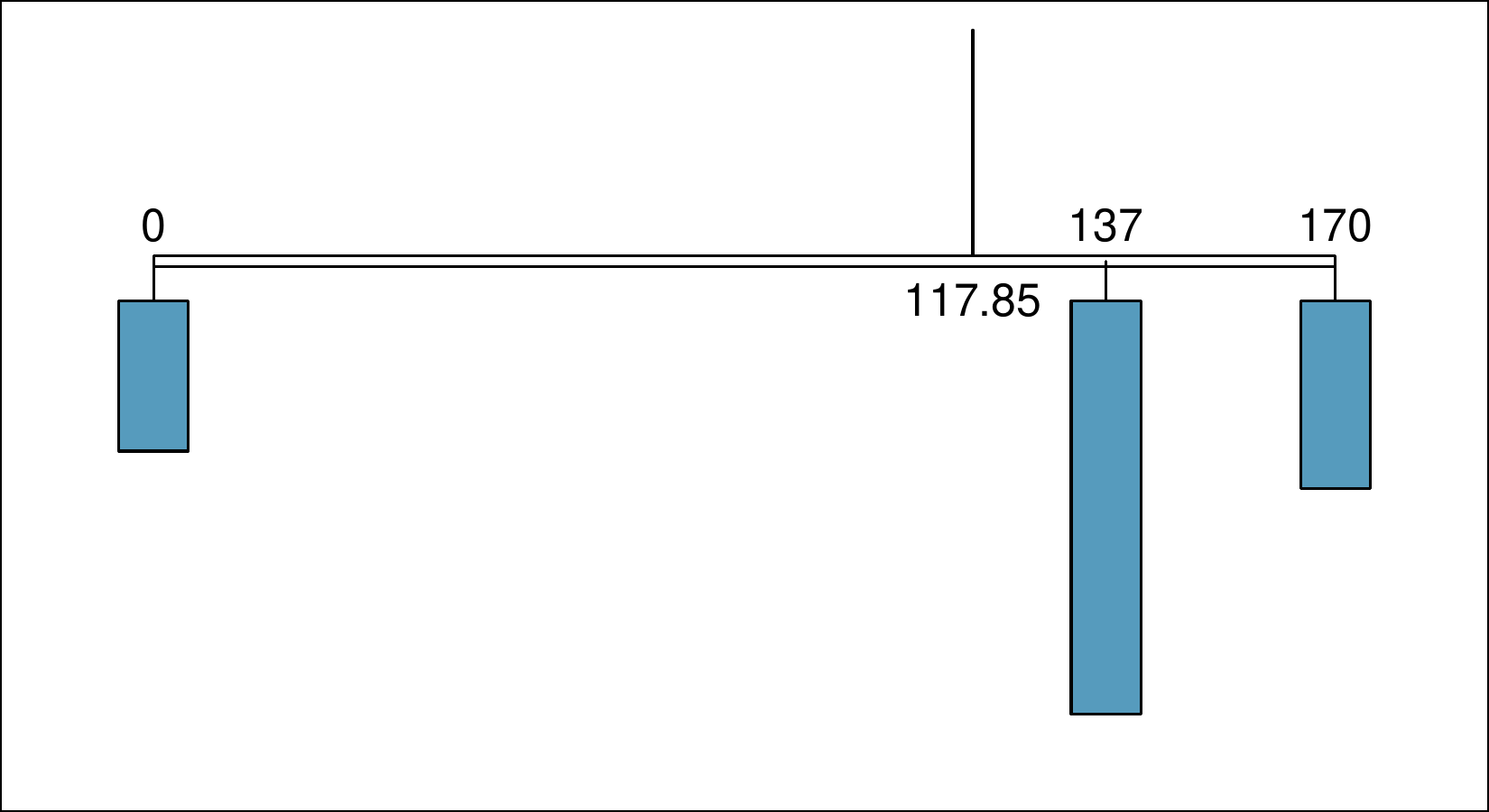
In physics, the expectation holds the same meaning as the center of gravity. The distribution can be represented by a series of weights at each outcome, and the mean represents the balancing point. This is represented in Figure 3.4.4 and Figure 3.4.6. The idea of a center of gravity also expands to continuous probability distributions. Figure 3.4.7 shows a continuous probability distribution balanced atop a wedge placed at the mean.

Figure 3.4.6. A weight system representing the probability distribution for $X\text{.}$ The string holds the distribution at the mean to keep the system balanced.

Figure 3.4.7. A continuous distribution can also be balanced at its mean.

Subsection 3.4.2 Variability in random variables

Suppose you ran the university bookstore. Besides how much revenue you expect to generate, you might also want to know the volatility (variability) in your revenue.

The variance and standard deviation can be used to describe the variability of a random variable. We first compute deviations from the mean ($x_i - \mu$), square those deviations, and take an average to get the variance. In the case of a random variable, we again compute squared deviations. However, we take their sum weighted by their corresponding probabilities, just like we did for the expectation. This weighted sum of squared deviations equals the variance, and we calculate the standard deviation by taking the square root of the variance.

Variance of a discrete random variable.

If $X$ takes outcomes $x_1, \ldots, x_k$ with probabilities $P(X=x_1), \ldots, P(X=x_k)$ and expected value $\mu = E(X)\text{,}$ then the variance of $X\text{,}$ denoted by $\text{Var}(X)$ or the symbol $\sigma^2\text{,}$ is

\begin{align*} \sigma^2 \amp= (x_1-\mu)^2 \times P(X=x_1) + \cdots + (x_k-\mu)^2 \times P(X=x_k)\\ \amp= \sum_{j=1}^{k} (x_j - \mu)^2 P(X=x_j) \end{align*}

The standard deviation of $X\text{,}$ labeled $\sigma\text{,}$ is the square root of the variance.

Example 3.4.8.

Compute the expected value, variance, and standard deviation of $X\text{,}$ the revenue of a single statistics student for the bookstore.

Solution.

It is useful to construct a table that holds computations for each outcome separately, then add up the results.

$i$	1	2	3	Total
$x_i$	$0	$137	$170
$P(X=x_i)$	0.20	0.55	0.25
$x_i \times P(X=x_i)$	0	75.35	42.50	117.85

Figure 3.4.9.

Thus, the expected value is $\mu = 117.85\text{,}$ which we computed earlier. The variance can be constructed by extending this table:

$i$	1	2	3	Total
$x_i$	$0	$137	$170
$P(X=x_i)$	0.20	0.55	0.25
$x_i \times P(X=x_i)$	0	75.35	42.50	117.85
$x_i - \mu$	-117.85	19.15	52.15
$(x_i-\mu)^2$	13888.62	366.72	2719.62
$(x_i-\mu)^2 \times P(X=x_i)$	2777.7	201.7	679.9	3659.3

Figure 3.4.10.

The variance of $X$ is $\sigma^2 = 3659.3\text{,}$ which means the standard deviation is $\sigma = \sqrt{3659.3} = \$60.49\text{.}$

Checkpoint 3.4.11.

The bookstore also offers a chemistry textbook for $159 and a book supplement for $41. From past experience, they know about 25% of chemistry students just buy the textbook while 60% buy both the textbook and supplement.

What proportion of students don’t buy either book? Assume no students buy the supplement without the textbook.
Let $Y$ represent the revenue from a single student. Write out the probability distribution of $Y\text{,}$ i.e. a table for each outcome and its associated probability.
Compute the expected revenue from a single chemistry student.
Find the standard deviation to describe the variability associated with the revenue from a single student.

Solution.

(a) $100\% - 25\% - 60\% = 15\%$ of students do not buy any books for the class.

(b) The probability distribution is represented in the table below.

(d) The result is the square root of the variance listed in the total on the last line: $\sigma = \sqrt{\text{Var}(Y)} = \$69.28\text{.}$

$i$	1	2	3	Total
Scenario	no book	textbook	both
$y_i$	0.00	159.00	200.00
$P(Y=y_i)$	0.15	0.25	0.60
$y_i \times P(Y=y_i)$	0.00	39.75	120.00	159.75
$y_i - E(Y)$	-159.75	-0.75	40.25
$(y_i-E(Y))^2$	25520.06	0.56	1620.06
$(y_i-E(Y))^2 \times P(Y)$	3828.0	0.1	972.0	$\approx 4800$

Figure 3.4.12.

Subsection 3.4.3 Linear combinations of random variables

So far, we have thought of each variable as being a complete story in and of itself. Sometimes it is more appropriate to use a combination of variables. For instance, the amount of time a person spends commuting to work each week can be broken down into several daily commutes. Similarly, the total gain or loss in a stock portfolio is the sum of the gains and losses in its components.

Example 3.4.13.

John travels to work five days a week. We will use $X_1$ to represent his travel time on Monday, $X_2$ to represent his travel time on Tuesday, and so on. Write an equation using $X_1, \ldots, X_5$ that represents his travel time for the week, denoted by $W\text{.}$

Solution.

His total weekly travel time is the sum of the five daily values:

\begin{equation*} W = X_1 + X_2 + X_3 + X_4 + X_5 \end{equation*}

Breaking the weekly travel time $W$ into pieces provides a framework for understanding each source of randomness and is useful for modeling $W\text{.}$

Example 3.4.14.

It takes John an average of 18 minutes each day to commute to work. What would you expect his average commute time to be for the week?

Solution.

We were told that the average (i.e. expected value) of the commute time is 18 minutes per day: $E(X_i) = 18\text{.}$ To get the expected time for the sum of the five days, we can add up the expected time for each individual day:

\begin{align*} E(W) \amp= E(X_1 + X_2 + X_3 + X_4 + X_5)\\ \amp= E(X_1) + E(X_2) + E(X_3) + E(X_4) + E(X_5)\\ \amp= 18 + 18 + 18 + 18 + 18 = 90 \text{ minutes} \end{align*}

The expectation of the total time is equal to the sum of the expected individual times. More generally, the expectation of a sum of random variables is always the sum of the expectation for each random variable.

Checkpoint 3.4.15.

Elena is selling a TV at a cash auction and also intends to buy a toaster oven in the auction. If $X$ represents the profit for selling the TV and $Y$ represents the cost of the toaster oven, write an equation that represents the net change in Elena’s cash.

Solution.

She will make $X$ dollars on the TV but spend $Y$ dollars on the toaster oven: $X - Y\text{.}$

Checkpoint 3.4.16.

Based on past auctions, Elena figures she should expect to make about $175 on the TV and pay about $23 for the toaster oven. In total, how much should she expect to make or spend?

Solution.

$E(X - Y) = E(X) - E(Y) = 175 - 23 = \$152\text{.}$ She should expect to make about $152.

Checkpoint 3.4.17.

Would you be surprised if John’s weekly commute wasn’t exactly 90 minutes or if Elena didn’t make exactly $152? Explain.

Solution.

No, since there is probably some variability. For example, the traffic will vary from one day to next, and auction prices will vary depending on the quality of the merchandise and the interest of the attendees.

Two important concepts concerning combinations of random variables have so far been introduced. First, a final value can sometimes be described as the sum of its parts in an equation. Second, intuition suggests that putting the individual average values into this equation gives the average value we would expect in total. This second point needs clarification -- it is guaranteed to be true in what are called linear combinations of random variables.

A linear combination of two random variables $X$ and $Y$ is a combination

\begin{equation*} aX + bY \end{equation*}

where $a$ and $b$ are some fixed and known numbers. For John’s commute time, there were five random variables -- one for each work day -- and each random variable could be written as having a fixed coefficient of 1:

\begin{equation*} 1X_1 + 1X_2 + 1X_3 + 1X_4 + 1X_5 \end{equation*}

For Elena’s net gain or loss, the $X$ random variable had a coefficient of +1 and the $Y$ random variable had a coefficient of -1.

When considering the average of a linear combination of random variables, it is safe to plug in the mean of each random variable and then compute the final result. For some examples of nonlinear combinations of random variables -- cases where we cannot simply plug in the means -- consider: $X^{1+Y}\text{,}$ $X \times Y\text{,}$ $X/Y\text{.}$ In such cases, plugging in the average value for each random variable and computing the result will not generally lead to an accurate average value for the end result.

Linear combinations of random variables and the average result.

If $X$ and $Y$ are random variables, then a linear combination of the random variables is given by

\begin{equation*} aX + bY \end{equation*}

where $a$ and $b$ are some fixed numbers. To compute the average value of a linear combination of random variables, plug in the average of each individual random variable and compute the result:

\begin{equation*} a \times E(X) + b \times E(Y) \end{equation*}

Recall that the expected value is the same as the mean, e.g. $E(X) = \mu_X\text{.}$

Example 3.4.18.

Leonard has invested $6000 in Caterpillar Inc (stock ticker: CAT) and $2000 in Exxon Mobil Corp (XOM). If $X$ represents the change in Caterpillar’s stock next month and $Y$ represents the change in Exxon Mobil’s stock next month, write an equation that describes how much money will be made or lost in Leonard’s stocks for the month.

Solution.

For simplicity, we will suppose $X$ and $Y$ are not in percents but are in decimal form (e.g. if Caterpillar’s stock increases 1%, then $X = 0.01\text{;}$ or if it loses 1%, then $X = -0.01$). Then we can write an equation for Leonard’s gain as

\begin{equation*} \$6000 \times X + \$2000 \times Y \end{equation*}

If we plug in the change in the stock value for $X$ and $Y\text{,}$ this equation gives the change in value of Leonard’s stock portfolio for the month. A positive value represents a gain, and a negative value represents a loss.

Checkpoint 3.4.19.

Caterpillar stock has recently been rising at 2.0% and Exxon Mobil’s at 0.2% per month, respectively. Compute the expected change in Leonard’s stock portfolio for next month.

Solution.

$E(\$6000 \times X + \$2000 \times Y) = \$6000 \times 0.020 + \$2000 \times 0.002 = \$124$

Checkpoint 3.4.20.

You should have found that Leonard expects a positive gain in Checkpoint 3.4.19. However, would you be surprised if he actually had a loss this month?

Solution.

No. While stocks tend to rise over time, they are often volatile in the short term.

Quantifying the average outcome from a linear combination of random variables is helpful, but it is also important to have some sense of the uncertainty associated with the total outcome of that combination of random variables. The expected net gain or loss of Leonard’s stock portfolio was considered in Checkpoint 3.4.19. However, there was no quantitative discussion of the volatility of this portfolio.

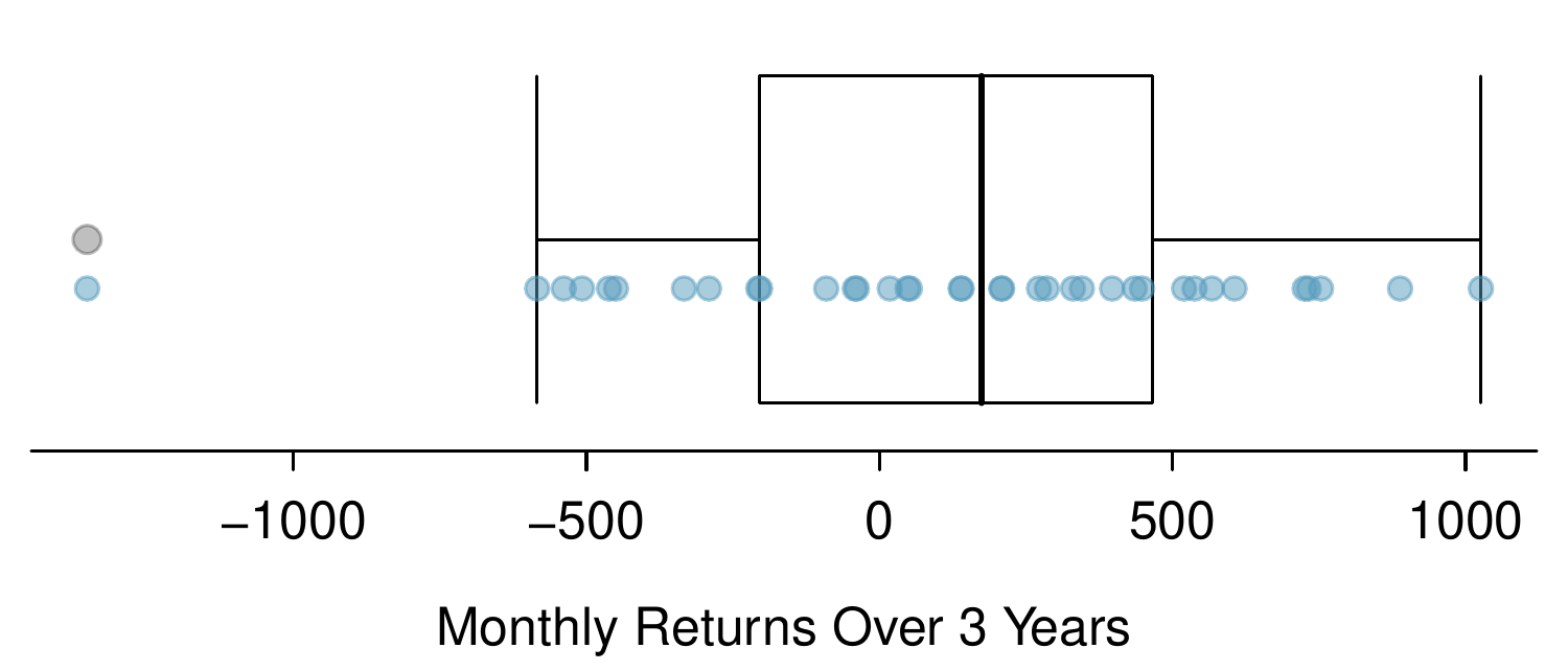
Figure 3.4.21. The change in a portfolio like Leonard’s for 36 months, where $6000 is in Caterpillar’s stock and $2000 is in Exxon Mobil’s.

For instance, while the average monthly gain might be about $124 according to the data, that gain is not guaranteed. The figure shows the monthly changes in a portfolio like Leonard’s during a three year period. The gains and losses vary widely, and quantifying these fluctuations is important when investing in stocks.

Just as we have done in many previous cases, we use the variance and standard deviation to describe the uncertainty associated with Leonard’s monthly returns. The variance of a linear combination of random variables can be computed by plugging in the variances of the individual random variables and squaring the coefficients of the random variables. This equation is valid as long as the random variables are independent.

Variability of linear combinations of random variables.

The variance of a linear combination of random variables may be computed by squaring the constants, substituting in the variances for the random variables, and computing the result:

\begin{equation*} \text{Var}(aX + bY) = a^2 \times \text{Var}(X) + b^2 \times \text{Var}(Y) \end{equation*}

This equation is valid as long as the random variables are independent of each other. The standard deviation of the linear combination may be found by taking the square root of the variance.

Example 3.4.22.

Suppose John’s daily commute has a standard deviation of 4 minutes. What is the uncertainty in his total commute time for the week?

Solution.

The expression for John’s commute time was

\begin{equation*} X_1 + X_2 + X_3 + X_4 + X_5 \end{equation*}

Each coefficient is 1, and the variance of each day’s time is $4^2 = 16\text{.}$ Thus, the variance of the total weekly commute time is

\begin{align*} \text{variance} \amp= 1^2 \times 16 + 1^2 \times 16 + 1^2 \times 16 + 1^2 \times 16 + 1^2 \times 16 = 5 \times 16 = 80\\ \text{standard deviation} \amp= \sqrt{\text{variance}} = \sqrt{80} = 8.94 \end{align*}

The standard deviation for John’s weekly work commute time is about 9 minutes.

Checkpoint 3.4.23.

The computation in Example 3.4.22 relied on an important assumption: the commute time for each day is independent of the time on other days of that week. Do you think this is valid? Explain.

Solution.

One concern is whether traffic patterns tend to have a weekly cycle (e.g. Fridays may be worse than other days). If that is the case, and John drives, then the assumption is probably not reasonable. However, if John walks to work, then his commute is probably not affected by any weekly traffic cycle.

Checkpoint 3.4.24.

Consider Elena’s two auctions from Checkpoint 3.4.15. Suppose these auctions are approximately independent and the variability in auction prices associated with the TV and toaster oven can be described using standard deviations of $25 and $8. Compute the standard deviation of Elena’s net gain.

Solution.

The equation for Elena can be written as

\begin{equation*} (1) \times X + (-1) \times Y \end{equation*}

The variances of $X$ and $Y$ are 625 and 64. We square the coefficients and plug in the variances:

\begin{equation*} (1)^2 \times \text{Var}(X) + (-1)^2 \times \text{Var}(Y) = 1 \times 625 + 1 \times 64 = 689 \end{equation*}

The variance of the linear combination is 689, and the standard deviation is the square root of 689: about $26.25.

Consider again Checkpoint 3.4.24. The negative coefficient for $Y$ in the linear combination was eliminated when we squared the coefficients. This generally holds true: negatives in a linear combination will have no impact on the variability computed for a linear combination, but they do impact the expected value computations.

Exercises 3.4.4 Exercises

1. College smokers.

At a university, 13% of students smoke.

Calculate the expected number of smokers in a random sample of 100 students from this university.
The university gym opens at 9 am on Saturday mornings. One Saturday morning at 8:55 am there are 27 students outside the gym waiting for it to open. Should you use the same approach from part (a) to calculate the expected number of smokers among these 27 students?

2. Ace of clubs wins.

Consider the following card game with a well-shuffled deck of cards. If you draw a red card, you win nothing. If you get a spade, you win $5. For any club, you win $10 plus an extra $20 for the ace of clubs.

Create a probability model for the amount you win at this game. Also, find the expected winnings for a single game and the standard deviation of the winnings.
What is the maximum amount you would be willing to pay to play this game? Explain your reasoning.

3. Hearts win.

In a new card game, you start with a well-shuffled full deck and draw 3 cards without replacement. If you draw 3 hearts, you win $50. If you draw 3 black cards, you win $25. For any other draws, you win nothing.

Create a probability model for the amount you win at this game, and find the expected winnings. Also compute the standard deviation of this distribution.
If the game costs $5 to play, what would be the expected value and standard deviation of the net profit (or loss)? (Hint: profit = winnings $-$ cost; $X-5$)
If the game costs $5 to play, should you play this game? Explain.

4. Is it worth it.

Andy is always looking for ways to make money fast. Lately, he has been trying to make money by gambling. Here is the game he is considering playing: The game costs $2 to play. He draws a card from a deck. If he gets a number card (2-10), he wins nothing. For any face card (jack, queen or king), he wins $3. For any ace, he wins $5, and he wins an extra $20 if he draws the ace of clubs.

Create a probability model and find Andy’s expected profit per game.
Would you recommend this game to Andy as a good way to make money? Explain.

5. Portfolio return.

A portfolio’s value increases by 18% during a financial boom and by 9% during normal times. It decreases by 12% during a recession. What is the expected return on this portfolio if each scenario is equally likely?

6. Baggage fees.

An airline charges the following baggage fees: $25 for the first bag and $35 for the second. Suppose 54% of passengers have no checked luggage, 34% have one piece of checked luggage and 12% have two pieces. We suppose a negligible portion of people check more than two bags.

Build a probability model, compute the average revenue per passenger, and compute the corresponding standard deviation.
About how much revenue should the airline expect for a flight of 120 passengers? With what standard deviation? Note any assumptions you make and if you think they are justified.

7. American roulette.

The game of American roulette involves spinning a wheel with 38 slots: 18 red, 18 black, and 2 green. A ball is spun onto the wheel and will eventually land in a slot, where each slot has an equal chance of capturing the ball. Gamblers can place bets on red or black. If the ball lands on their color, they double their money. If it lands on another color, they lose their money. Suppose you bet $1 on red. What’s the expected value and standard deviation of your winnings?

8. European roulette.

The game of European roulette involves spinning a wheel with 37 slots: 18 red, 18 black, and 1 green. A ball is spun onto the wheel and will eventually land in a slot, where each slot has an equal chance of capturing the ball. Gamblers can place bets on red or black. If the ball lands on their color, they double their money. If it lands on another color, they lose their money.

Suppose you play roulette and bet $3 on a single round. What is the expected value and standard deviation of your total winnings?
Suppose you bet $1 in three different rounds. What is the expected value and standard deviation of your total winnings?
How do your answers to parts (a) and (b) compare? What does this say about the riskiness of the two games?

Prev Top Next

\(i\)	1	2	3	Total
\(x_i\)	$0	$137	$170	--
\(P(X=x_i)\)	0.20	0.55	0.25	1.00