We encountered inference methods for a single proportion in Chapter 5, exploring point estimates, confidence intervals, and hypothesis tests. In this section, we’ll do a review of these topics and also how to choose an appropriate sample size when collecting data for single proportion contexts.
Subsection6.1.1Identifying when the sample proportion is nearly normal
A sample proportion \(\hat{p}\) can be modeled using a normal distribution when the sample observations are independent and the sample size is sufficiently large.
When these conditions are met, then the sampling distribution of \(\hat{p}\) is nearly normal with mean \(p\) and standard error \(SE = \sqrt{\frac{p(1-p)}{n}}\text{.}\)
Typically we don’t know the true proportion \(p\text{,}\) so we substitute some value to check conditions and estimate the standard error. For confidence intervals, the sample proportion \(\hat{p}\) is used to check the success-failure condition and compute the standard error. For hypothesis tests, typically the null value—that is, the proportion claimed in the null hypothesis—is used in place of \(p\text{.}\)
Subsection6.1.2Confidence intervals for a proportion
A confidence interval provides a range of plausible values for the parameter \(p\text{,}\) and when \(\hat{p}\) can be modeled using a normal distribution, the confidence interval for \(p\) takes the form
\begin{equation*}
\hat{p} \pm z^{\star} \times SE
\end{equation*}
Example6.1.1.
A simple random sample of 826 payday loan borrowers was surveyed to better understand their interests around regulation and costs. 70% of the responses supported new regulations on payday lenders. Is it reasonable to model \(\hat{p} = 0.70\) using a normal distribution?
Estimate the standard error of \(\hat{p} = 0.70\text{.}\) Because \(p\) is unknown and the standard error is for a confidence interval, use \(\hat{p}\) in place of \(p\) in the formula.
Using the point estimate 0.70, \(z^{\star} = 1.96\) for a 95% confidence interval, and the standard error \(SE = 0.016\) from Guided Practice Checkpoint 6.1.2, the confidence interval is
Verify the conditions to ensure \(\hat{p}\) is nearly normal. For one-proportion confidence intervals, use \(\hat{p}\) in place of \(p\) to check the success-failure condition.
Subsection6.1.3Hypothesis testing for a proportion
One possible regulation for payday lenders is that they would be required to do a credit check and evaluate debt payments against the borrower’s finances. We would like to know: would borrowers support this form of regulation?
To apply the normal distribution framework in the context of a hypothesis test for a proportion, the independence and success-failure conditions must be satisfied. In a hypothesis test, the success-failure condition is checked using the null proportion: we verify \(np_0\) and \(n(1-p_0)\) are at least 10, where \(p_0\) is the null value.
Do payday loan borrowers support a regulation that would require lenders to pull their credit report and evaluate their debt payments? From a random sample of 826 borrowers, 51% said they would support such a regulation. Is it reasonable to model \(\hat{p} = 0.51\) using a normal distribution for a hypothesis test here?
Independence holds since the poll is based on a random sample. The success-failure condition also holds, which is checked using the null value (\(p_0 = 0.5\)) from \(H_0\text{:}\)\(np_0 = 826 \times 0.5 = 413\text{,}\)\(n(1 - p_0) = 826 \times 0.5 = 413\text{.}\)
Using the hypotheses and data from Checkpoint 6.1.4 and Checkpoint 6.1.5, evaluate whether the poll provides convincing evidence that a majority of payday loan borrowers support a new regulation that would require lenders to pull credit reports and evaluate debt payments.
With hypotheses already set up and conditions checked, we can move onto calculations. The standard error in the context of a one-proportion hypothesis test is computed using the null value, \(p_0\text{:}\)
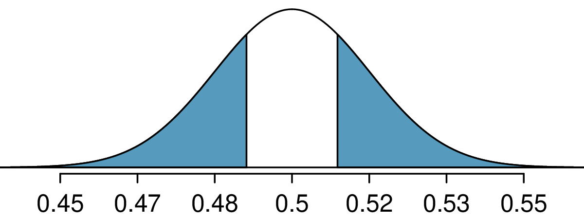
Figure6.1.7.A normal distribution is shown with a center of 0.5 and a standard deviation of 0.017. Two tails are shaded: The region above 0.51 and a region in the corresponding lower tail. Visually, it looks like a little over half of the area under the normal curve is shaded.
The single tail area is 0.2776, and the p-value, represented by both tail areas together, is 0.5552. Because the p-value is larger than 0.05, we do not reject \(H_0\text{.}\) The poll does not provide convincing evidence that a majority of payday loan borrowers support or oppose regulations around credit checks and evaluation of debt payments.
Verify conditions to ensure \(\hat{p}\) is nearly normal under \(H_0\text{.}\) For one-proportion hypothesis tests, use the null value to check the success-failure condition.
Subsection6.1.4When one or more conditions aren’t met
We’ve spent a lot of time discussing conditions for when \(\hat{p}\) can be reasonably modeled by a normal distribution. What happens when the success-failure condition fails? What about when the independence condition fails? In either case, the general ideas of confidence intervals and hypothesis tests remain the same, but the strategy or technique used to generate the interval or p-value change.
When the success-failure condition isn’t met for a hypothesis test, we can simulate the null distribution of \(\hat{p}\) using the null value, \(p_0\text{.}\) The simulation concept is similar to the ideas used in the malaria case study presented in 5.1, and an online section by OpenIntro outlines this strategy: www.openintro.org/r?go=stat_sim_prop_ht
For a confidence interval when the success-failure condition isn’t met, we can use what’s called the Clopper-Pearson interval. The details are beyond the scope of this book. However, there are many internet resources covering this topic.
The independence condition is a more nuanced requirement. When it isn’t met, it is important to understand how and why it isn’t met. For example, if we took a cluster sample (see 1.3), suitable statistical methods are available but would be beyond the scope of even most second or third courses in statistics. On the other hand, we’d be stretched to find any method that we could confidently apply to correct the inherent biases of data from a convenience sample.
While this book is scoped to well-constrained statistical problems, do remember that this is just the first book in what is a large library of statistical methods that are suitable for a very wide range of data and contexts.
Subsection6.1.5Choosing a sample size when estimating a proportion
When collecting data, we choose a sample size suitable for the purpose of the study. Often times this means choosing a sample size large enough that the margin of error—which is the part we add and subtract from the point estimate in a confidence interval—is sufficiently small that the sample is useful. For example, our task might be to find a sample size \(n\) so that the sample proportion is within \(\pm 0.04\) of the actual proportion in a 95% confidence interval.
A university newspaper is conducting a survey to determine what fraction of students support a $200 per year increase in fees to pay for a new football stadium. How big of a sample is required to ensure the margin of error is smaller than 0.04 using a 95% confidence level?
Our goal is to find the smallest sample size \(n\) so that this margin of error is smaller than 0.04. For a 95% confidence level, the value \(z^{\star}\) corresponds to 1.96:
There are two unknowns in the equation: \(p\) and \(n\text{.}\) If we have an estimate of \(p\text{,}\) perhaps from a prior survey, we could enter in that value and solve for \(n\text{.}\) If we have no such estimate, we must use some other value for \(p\text{.}\) It turns out that the margin of error is largest when \(p\) is 0.5, so we typically use this worst case value if no estimate of the proportion is available:
We would need over 600.25 participants, which means we need 601 participants or more, to ensure the sample proportion is within 0.04 of the true proportion with 95% confidence.
A manager is about to oversee the mass production of a new tire model in her factory, and she would like to estimate what proportion of these tires will be rejected through quality control. The quality control team has monitored the last three tire models produced by the factory, failing 1.7% of tires in the first model, 6.2% of the second model, and 1.3% of the third model. The manager would like to examine enough tires to estimate the failure rate of the new tire model to within about 1% with a 90% confidence level. There are three different failure rates to choose from. Perform the sample size computation for each separately, and identify three sample sizes to consider.
For a 90% confidence interval, \(z^{\star} = 1.6449\text{,}\) and since an estimate of the proportion 0.017 is available, we’ll use it in the margin of error formula:
A similar computation can be accomplished using 0.062 and 0.013 for \(p\text{,}\) and you should verify that using these proportions results in minimum sample sizes of 1574 and 348 tires, respectively.
We could examine which of the old models is most like the new model, then choose the corresponding sample size. Or if two of the previous estimates are based on small samples while the other is based on a larger sample, we might consider the value corresponding to the larger sample. There are also other reasonable approaches.
Also observe that the success-failure condition would need to be checked in the final sample. For instance, if we sampled \(n = 1584\) tires and found a failure rate of 0.5%, the normal approximation would not be reasonable, and we would require more advanced statistical methods for creating the confidence interval.
Suppose we want to continually track the support of payday borrowers for regulation on lenders, where we would conduct a new poll every month. Running such frequent polls is expensive, so we decide a wider margin of error of 5% for each individual survey would be acceptable. Based on the original sample of borrowers where 70% supported some form of regulation, how big should our monthly sample be for a margin of error of 0.05 with 95% confidence?
A sample size of 323 or more would be reasonable. (Reminder: always round up for sample size calculations!) Given that we plan to track this poll over time, we also may want to periodically repeat these calculations to ensure that we’re being thoughtful in our sample size recommendations in case the baseline rate fluctuates.
About 77% of young adults think they can achieve the American dream. Determine if the following statements are true or false, and explain your reasoning.
The distribution of sample proportions of young Americans who think they can achieve the American dream in random samples of size 40 is approximately normal since \(n \geq 30\text{.}\)
About 25% of young Americans have delayed starting a family due to the continued economic slump. Determine if the following statements are true or false, and explain your reasoning.
The distribution of sample proportions of young Americans who have delayed starting a family due to the continued economic slump in random samples of size 12 is right skewed.
In order for the distribution of sample proportions of young Americans who have delayed starting a family due to the continued economic slump to be approximately normal, we need random samples where the sample size is at least 40.
The General Social Survey asked a random sample of 1,390 Americans the following question: "On the whole, do you think it should or should not be the government’s responsibility to promote equality between men and women?" 82% of the respondents said it "should be". At a 95% confidence level, this sample has 2% margin of error. Based on this information, determine if the following statements are true or false, and explain your reasoning.
We are 95% confident that between 80% and 84% of Americans in this sample think it’s the government’s responsibility to promote equality between men and women.
If we considered many random samples of 1,390 Americans, and we calculated 95% confidence intervals for each, 95% of these intervals would include the true population proportion of Americans who think it’s the government’s responsibility to promote equality between men and women.
Based on this confidence interval, there is sufficient evidence to conclude that a majority of Americans think it’s the government’s responsibility to promote equality between men and women.
The Marist Poll published a report stating that 66% of adults nationally think licensed drivers should be required to retake their road test once they reach 65 years of age. It was also reported that interviews were conducted on 1,018 American adults, and that the margin of error was 3% using a 95% confidence level.
Based on a 95% confidence interval, does the poll provide convincing evidence that more than 70% of the population think that licensed drivers should be required to retake their road test once they turn 65?
A local news outlet reported that 56% of 600 randomly sampled Kansas residents planned to set off fireworks on July \(4^\text{th}\text{.}\) Determine the margin of error for the 56% point estimate using a 95% confidence level.
Greece has faced a severe economic crisis since the end of 2009. A Gallup poll surveyed 1,000 randomly sampled Greeks in 2011 and found that 25% of them said they would rate their lives poorly enough to be considered "suffering".
A survey on 1,509 high school seniors who took the SAT and who completed an optional web survey shows that 55% of high school seniors are fairly certain that they will participate in a study abroad program in college.
Let’s suppose the conditions for inference are met. Even if your answer to part (a) indicated that this approach would not be reliable, this analysis may still be interesting to carry out (though not report). Construct a 90% confidence interval for the proportion of high school seniors (of those who took the SAT) who are fairly certain they will participate in a study abroad program in college, and interpret this interval in context.
Based on this interval, would it be appropriate to claim that the majority of high school seniors are fairly certain that they will participate in a study abroad program in college?
The General Social Survey asked 1,578 US residents: "Do you think the use of marijuana should be made legal, or not?" 61% of the respondents said it should be made legal.
Construct a 95% confidence interval for the proportion of US residents who think marijuana should be made legal, and interpret it in the context of the data.
A critic points out that this 95% confidence interval is only accurate if the statistic follows a normal distribution, or if the normal model is a good approximation. Is this true for these data? Explain.
A news piece on this survey’s findings states, "Majority of Americans think marijuana should be legalized." Based on your confidence interval, is this news piece’s statement justified?
A Kaiser Family Foundation poll for US adults in 2019 found that 79% of Democrats, 55% of Independents, and 24% of Republicans supported a generic "National Health Plan". There were 347 Democrats, 298 Republicans, and 617 Independents surveyed.
A political pundit on TV claims that a majority of Independents support a National Health Plan. Do these data provide strong evidence to support this type of statement?
Among a simple random sample of 331 American adults who do not have a four-year college degree and are not currently enrolled in school, 48% said they decided not to go to college because they could not afford school.
A newspaper article states that only a minority of the Americans who decide not to go to college do so because they cannot afford it and uses the point estimate from this survey as evidence. Conduct a hypothesis test to determine if these data provide strong evidence supporting this statement.
Would you expect a confidence interval for the proportion of American adults who decide not to go to college because they cannot afford it to include 0.5? Explain.
Some people claim that they can tell the difference between a diet soda and a regular soda in the first sip. A researcher wanting to test this claim randomly sampled 80 such people. He then filled 80 plain white cups with soda, half diet and half regular through random assignment, and asked each person to take one sip from their cup and identify the soda as diet or regular. 53 participants correctly identified the soda.
Do these data provide strong evidence that these people are any better or worse than random guessing at telling the difference between diet and regular soda?
Calculate a 90% confidence interval for the proportion of Americans who decide to not go to college because they cannot afford it, and interpret the interval in context.
Exercise 6.1.6.11 presents the results of a poll evaluating support for a generic "National Health Plan" in the US in 2019, reporting that 55% of Independents are supportive. If we wanted to estimate this number to within 1% with 90% confidence, what would be an appropriate sample size?
As discussed in Exercise 6.1.6.10, the General Social Survey reported a sample where about 61% of US residents thought marijuana should be made legal. If we wanted to limit the margin of error of a 95% confidence interval to 2%, about how many Americans would we need to survey?