Testing for goodness of fit using chi-square

Section 6.3 Testing for goodness of fit using chi-square

In this section, we develop a method for assessing a null model when the data are binned. This technique is commonly used in two circumstances:

🔗

Given a sample of cases that can be classified into several groups, determine if the sample is representative of the general population.

🔗
Evaluate whether data resemble a particular distribution, such as a normal distribution or a geometric distribution.

🔗

Each of these scenarios can be addressed using the same statistical test: a chi-square test.

🔗

In the first case, we consider data from a random sample of 275 jurors in a small county. Jurors identified their racial group, as shown in Table 6.3.1, and we would like to determine if these jurors are racially representative of the population. If the jury is representative of the population, then the proportions in the sample should roughly reflect the population of eligible jurors, i.e. registered voters.

🔗

Table 6.3.1. Representation by race in a city’s juries and population.

🔗

Race	White	Black	Hispanic	Other	Total
Representation in juries	205	26	25	19	275
Registered voters	0.72	0.07	0.12	0.09	1.00

While the proportions in the juries do not precisely represent the population proportions, it is unclear whether these data provide convincing evidence that the sample is not representative. If the jurors really were randomly sampled from the registered voters, we might expect small differences due to chance. However, unusually large differences may provide convincing evidence that the juries were not representative.

🔗

A second application, assessing the fit of a distribution, is presented at the end of this section. Daily stock returns from the S&P500 for 25 years are used to assess whether stock activity each day is independent of the stock’s behavior on previous days.

🔗

In these problems, we would like to examine all bins simultaneously, not simply compare one or two bins at a time, which will require us to develop a new test statistic.

🔗

Subsection 6.3.1 Creating a test statistic for one-way tables

Example 6.3.2.

Of the people in the city, 275 served on a jury. If the individuals are randomly selected to serve on a jury, about how many of the 275 people would we expect to be White? How many would we expect to be Black?

🔗

Solution.

About 72% of the population is White, so we would expect about 72% of the jurors to be White: \(0.72\times 275 = 198\text{.}\)

🔗

Similarly, we would expect about 7% of the jurors to be Black, which would correspond to about \(0.07\times 275 = 19.25\) Black jurors.

🔗

Checkpoint 6.3.3.

Twelve percent of the population is Hispanic and 9% represent other races. How many of the 275 jurors would we expect to be Hispanic or from another race? Answers can be found in Table 6.3.4.

🔗

Solution.

Hispanic: \(0.12 \times 275 = 33\text{.}\) Other: \(0.09 \times 275 = 24.75\text{.}\)

🔗

Table 6.3.4. Actual and expected make-up of the jurors.

🔗

Race	White	Black	Hispanic	Other	Total
Observed data	205	26	25	19	275
Expected counts	198	19.25	33	24.75	275

The sample proportion represented from each race among the 275 jurors was not a precise match for any ethnic group. While some sampling variation is expected, we would expect the sample proportions to be fairly similar to the population proportions if there is no bias on juries. We need to test whether the differences are strong enough to provide convincing evidence that the jurors are not a random sample. These ideas can be organized into hypotheses:

🔗

\(H_0\text{:}\) The jurors are a random sample, i.e. there is no racial bias in who serves on a jury, and the observed counts reflect natural sampling fluctuation.

🔗
\(H_A\text{:}\) The jurors are not randomly sampled, i.e. there is racial bias in juror selection.

🔗

To evaluate these hypotheses, we quantify how different the observed counts are from the expected counts. Strong evidence for the alternative hypothesis would come in the form of unusually large deviations in the groups from what would be expected based on sampling variation alone.

🔗

Subsection 6.3.2 The chi-square test statistic

In previous hypothesis tests, we constructed a test statistic of the following form:

🔗

\begin{equation*} \frac{\text{point estimate} - \text{null value}}{\text{SE of point estimate}} \end{equation*}

This construction was based on (1) identifying the difference between a point estimate and an expected value if the null hypothesis was true, and (2) standardizing that difference using the standard error of the point estimate. These two ideas will help in the construction of an appropriate test statistic for count data.

🔗

Our strategy will be to first compute the difference between the observed counts and the counts we would expect if the null hypothesis was true, then we will standardize the difference:

🔗

\begin{equation*} Z_{1} = \frac{\text{observed White count} - \text{null White count}}{\text{SE of observed White count}} \end{equation*}

The standard error for the point estimate of the count in binned data is the square root of the count under the null.

Using some of the rules learned in earlier chapters, we might think that the standard error would be \(np(1-p)\text{,}\) where \(n\) is the sample size and \(p\) is the proportion in the population. This would be correct if we were looking only at one count. However, we are computing many standardized differences and adding them together. It can be shown—though not here—that the square root of the count is a better way to standardize the count differences.

Therefore:

🔗

\begin{equation*} Z_1 = \frac{205 - 198}{\sqrt{198}} = 0.50 \end{equation*}

The fraction is very similar to previous test statistics: first compute a difference, then standardize it. These computations should also be completed for the Black, Hispanic, and other groups:

🔗

\begin{align*} \text{Black} \qquad Z_2 \amp = \frac{26-19.25}{\sqrt{19.25}}=1.54\\ \text{Hispanic} \qquad Z_3 \amp = \frac{25-33}{\sqrt{33}}=-1.39\\ \text{Other} \qquad Z_4 \amp = \frac{19-24.75}{\sqrt{24.75}}=-1.16 \end{align*}

We would like to use a single test statistic to determine if these four standardized differences are irregularly far from zero. That is, \(Z_1\text{,}\) \(Z_2\text{,}\) \(Z_3\text{,}\) and \(Z_4\) must be combined somehow to help determine if they—as a group—tend to be unusually far from zero. A first thought might be to take the absolute value of these four standardized differences and add them up:

🔗

\begin{equation*} |Z_1| + |Z_2| + |Z_3| + |Z_4| = 4.58 \end{equation*}

Indeed, this does give one number summarizing how far the actual counts are from what was expected. However, it is more common to add the squared values:

🔗

\begin{equation*} Z_1^2 + Z_2^2 + Z_3^2 + Z_4^2 = 5.89 \end{equation*}

Squaring each standardized difference before adding them together does two things:

🔗

Any standardized difference that is squared will now be positive.

🔗
Differences that already look unusual—e.g. a standardized difference of 2.5—will become much larger after being squared.

🔗

The test statistic \(X^2\text{,}\) which is the sum of the \(Z^2\) values, is generally used for these reasons. We can also write an equation for \(X^2\) using the observed counts and null counts:

🔗

\begin{equation*} X^2 = \frac{(\text{observed count}_1 - \text{null count}_1)^2}{\text{null count}_1} + \dots + \frac{(\text{observed count}_4 - \text{null count}_4)^2}{\text{null count}_4} \end{equation*}

The final number \(X^2\) summarizes how strongly the observed counts tend to deviate from the null counts. In Subsection 6.3.4, we will see that if the null hypothesis is true, then \(X^2\) follows a new distribution called a chi-square distribution. Using this distribution, we will be able to obtain a p-value to evaluate the hypotheses.

🔗

Subsection 6.3.3 The chi-square distribution and finding areas

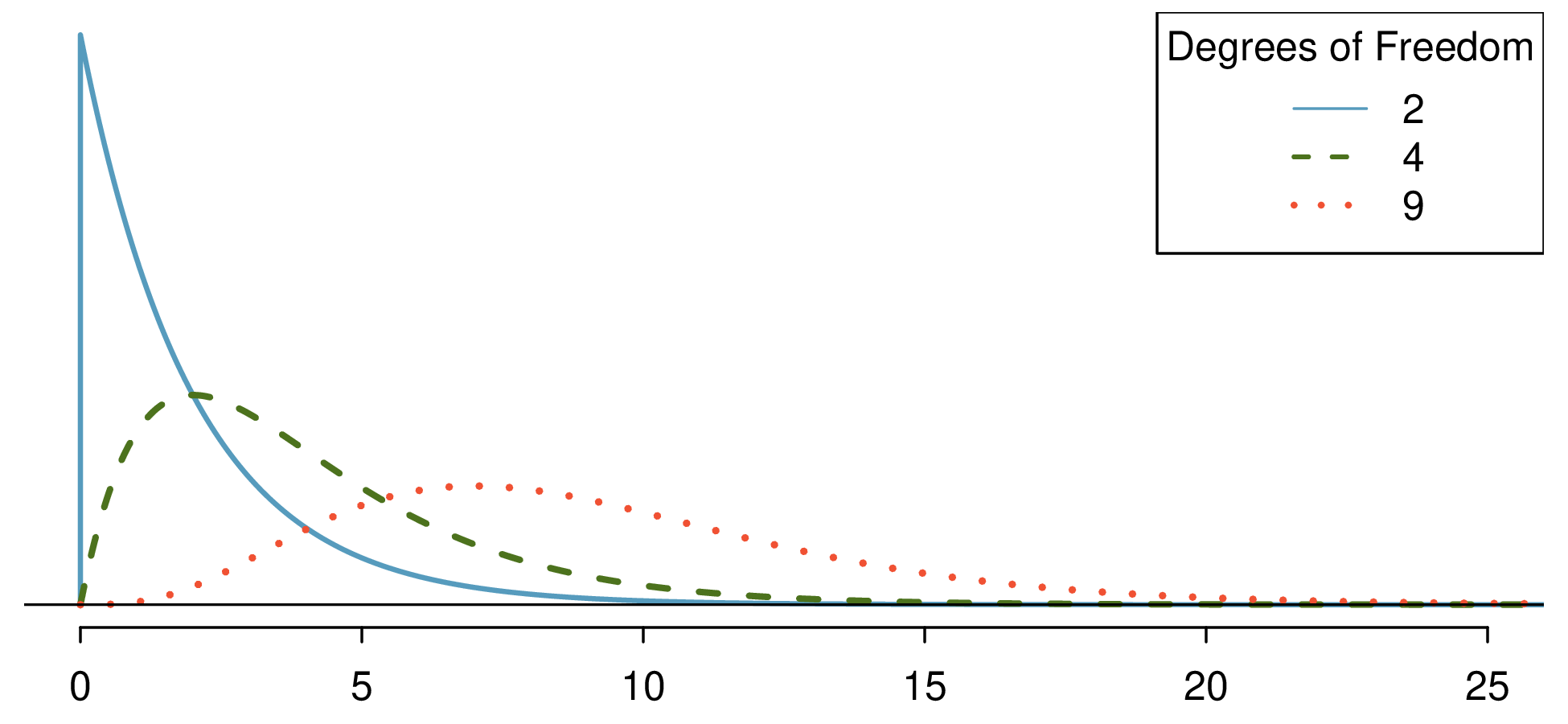
The chi-square distribution is sometimes used to characterize data sets and statistics that are always positive and typically right skewed. Recall a normal distribution had two parameters—mean and standard deviation—that could be used to describe its exact characteristics. The chi-square distribution has just one parameter called degrees of freedom (df), which influences the shape, center, and spread of the distribution.

🔗

Checkpoint 6.3.5.

Figure 6.3.6 shows three chi-square distributions.

🔗

(a) How does the center of the distribution change when the degrees of freedom is larger?

🔗

(b) What about the variability (spread)?

🔗

Solution.

(a) The center becomes larger. If took a careful look, we could see that the mean of each distribution is equal to the distribution’s degrees of freedom.

🔗

(b) The variability increases as the degrees of freedom increases.

🔗

(c) The distribution is very strongly skewed for \(df=2\text{,}\) and then the distributions become more symmetric for the larger degrees of freedom \(df=4\) and \(df=9\text{.}\) We would see this trend continue if we examined distributions with even more larger degrees of freedom.

🔗

described in detail following the image — Figure 6.3.6. Three chi-square distributions with varying degrees of freedom.
🔗

Figure 6.3.6 and Checkpoint 6.3.5 demonstrate three general properties of chi-square distributions as the degrees of freedom increases: the distribution becomes more symmetric, the center moves to the right, and the variability inflates.

🔗

Our principal interest in the chi-square distribution is the calculation of p-values, which (as we have seen before) is related to finding the relevant area in the tail of a distribution. The most common ways to do this are using computer software, using a graphing calculator, or using a table. For folks wanting to use the table option, we provide an outline of how to read the chi-square table in Appendix C, which is also where you may find the table. For the examples below, use your preferred approach to confirm you get the same answers.

🔗

Example 6.3.7.

Figure 6.3.8(a) shows a chi-square distribution with 3 degrees of freedom and an upper shaded tail starting at 6.25. Find the shaded area.

🔗

Solution.

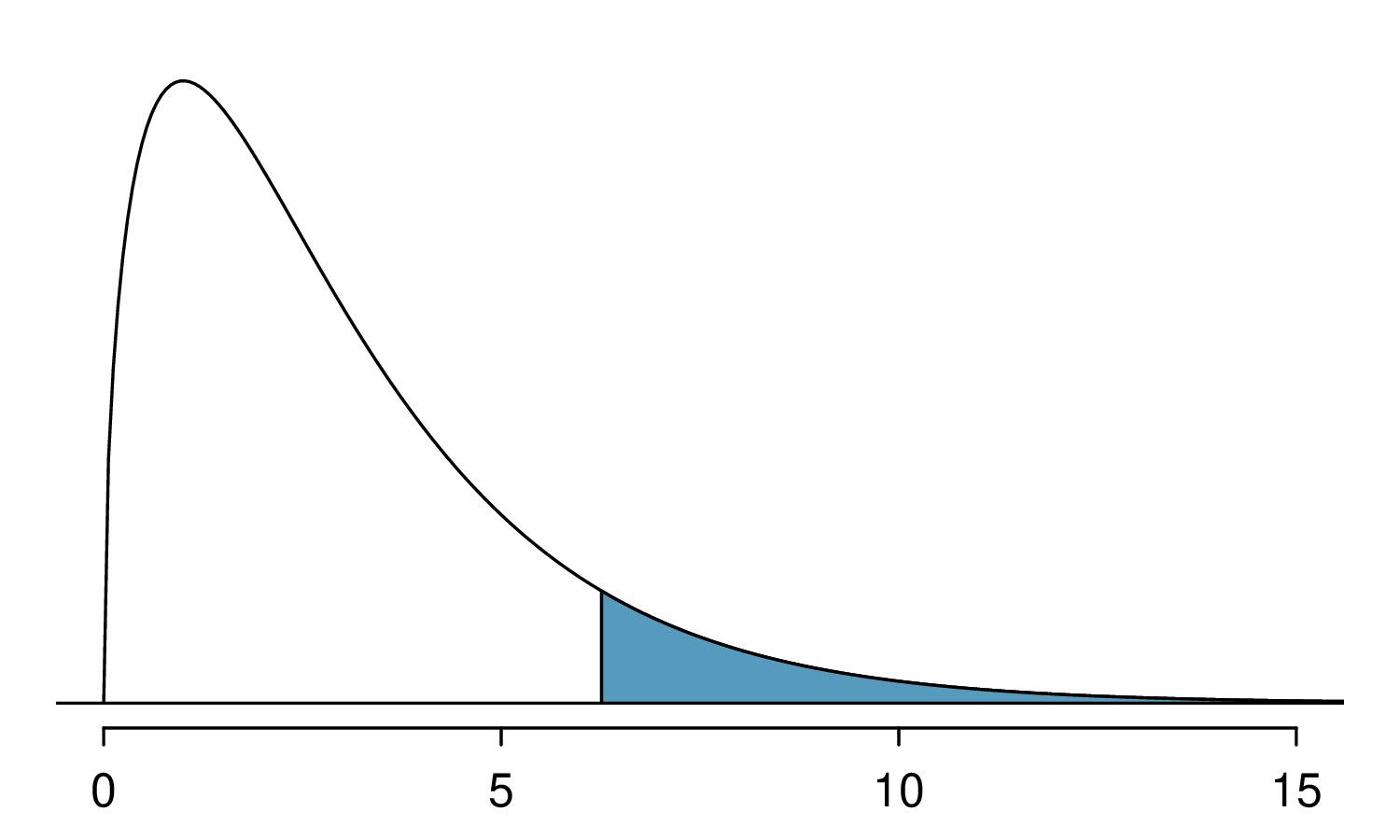
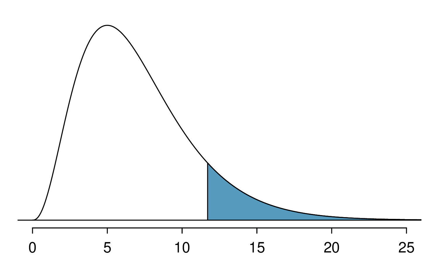
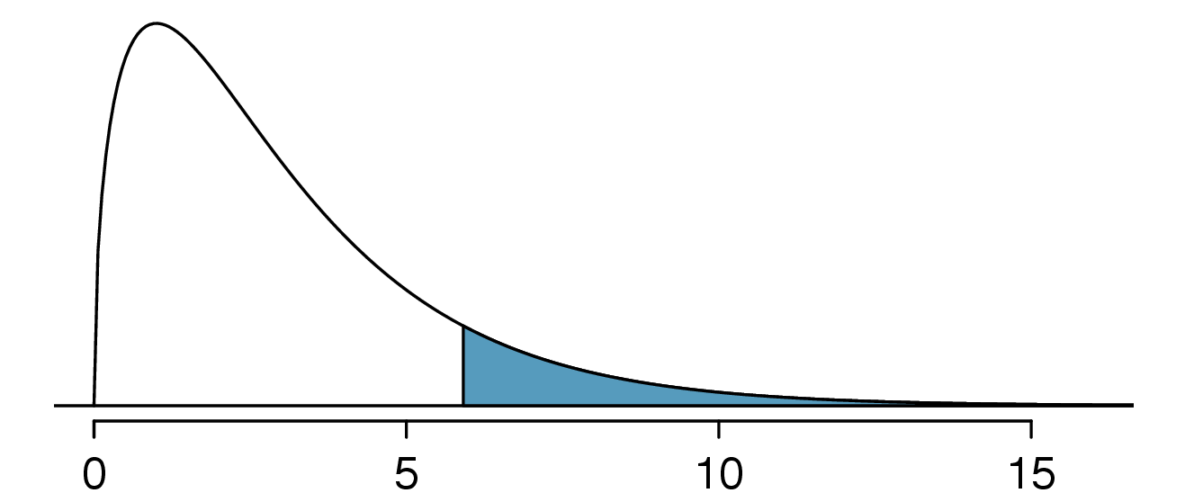
Using statistical software or a graphing calculator, we can find that the upper tail area for a chi-square distribution with 3 degrees of freedom (\(df\)) and a cutoff of 6.25 is 0.1001. That is, the shaded upper tail of Figure 6.3.8(a) has area 0.1.

🔗

A chi-square distribution with 3 degrees of freedom is shown, with the area above 6.25 shaded. This region appears to be about 10% of the area under the curve. — (a) Chi-square distribution with 3 degrees of freedom, area above 6.25 shaded.
🔗

A chi-square distribution with 2 degrees of freedom is shown, with the area above 4.3 shaded. This region appears to be about 10% of the area under the curve. — (a) Chi-square distribution with 3 degrees of freedom, area above 6.25 shaded.
🔗

Example 6.3.9.

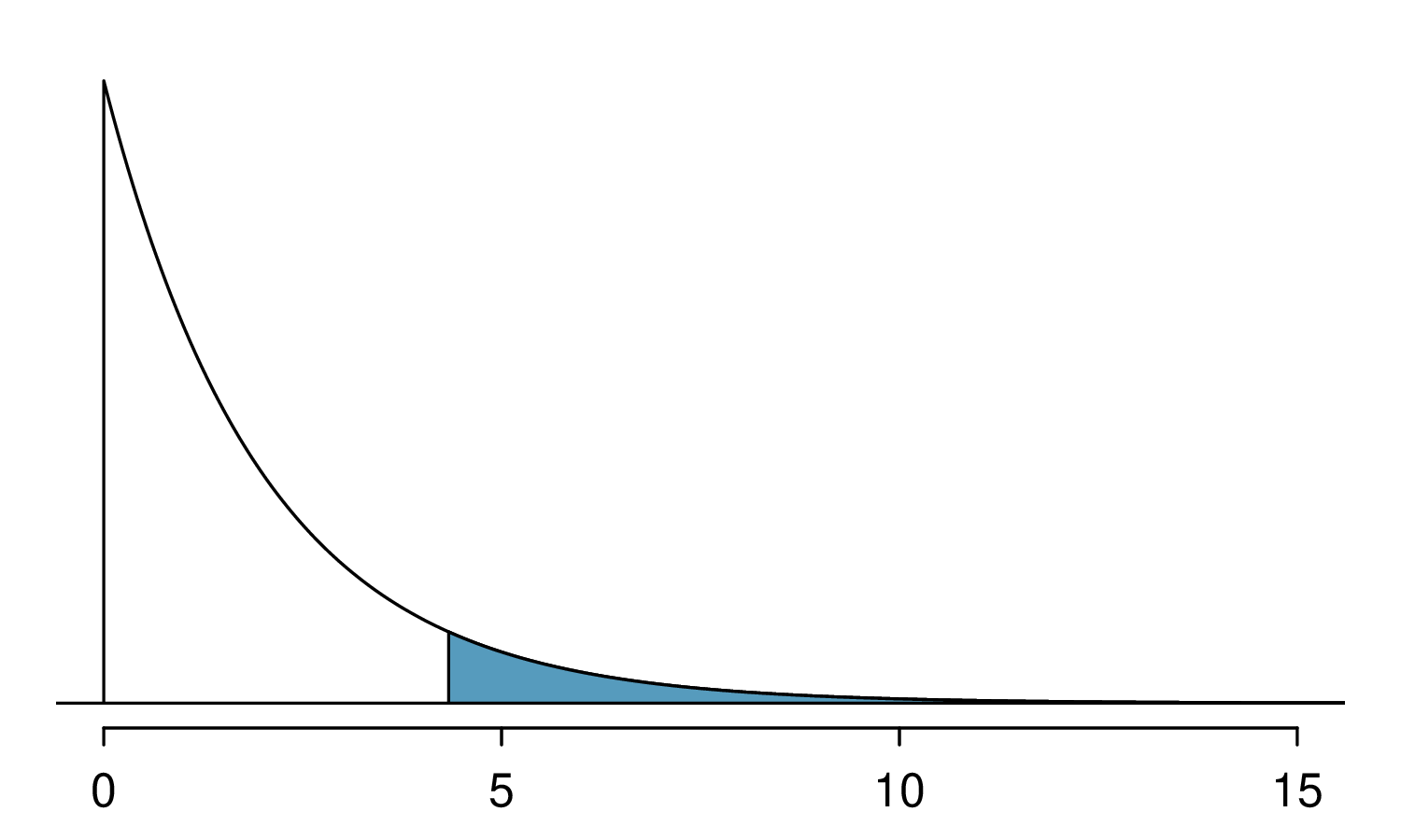
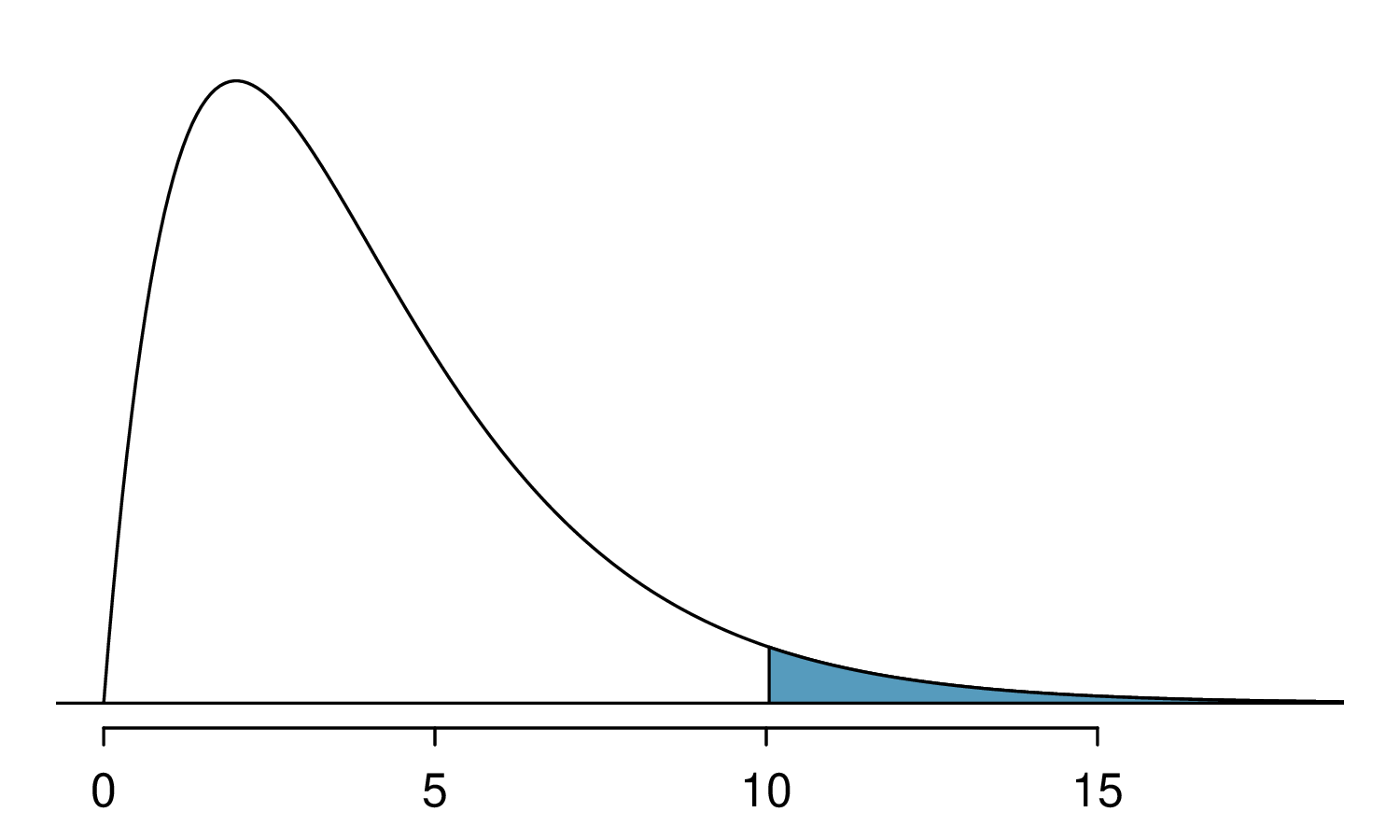
Figure 6.3.8(b) shows the upper tail of a chi-square distribution with 2 degrees of freedom. The bound for this upper tail is at 4.3. Find the tail area.

🔗

Solution.

Using software, we can find that the tail area shaded in Figure 6.3.8(b) to be 0.1165. If using a table, we would only be able to find a range of values for the tail area: between 0.1 and 0.2.

🔗

Example 6.3.10.

Figure 6.3.8(a) shows an upper tail for a chi-square distribution with 5 degrees of freedom and a cutoff of 5.1. Find the tail area.

🔗

Solution.

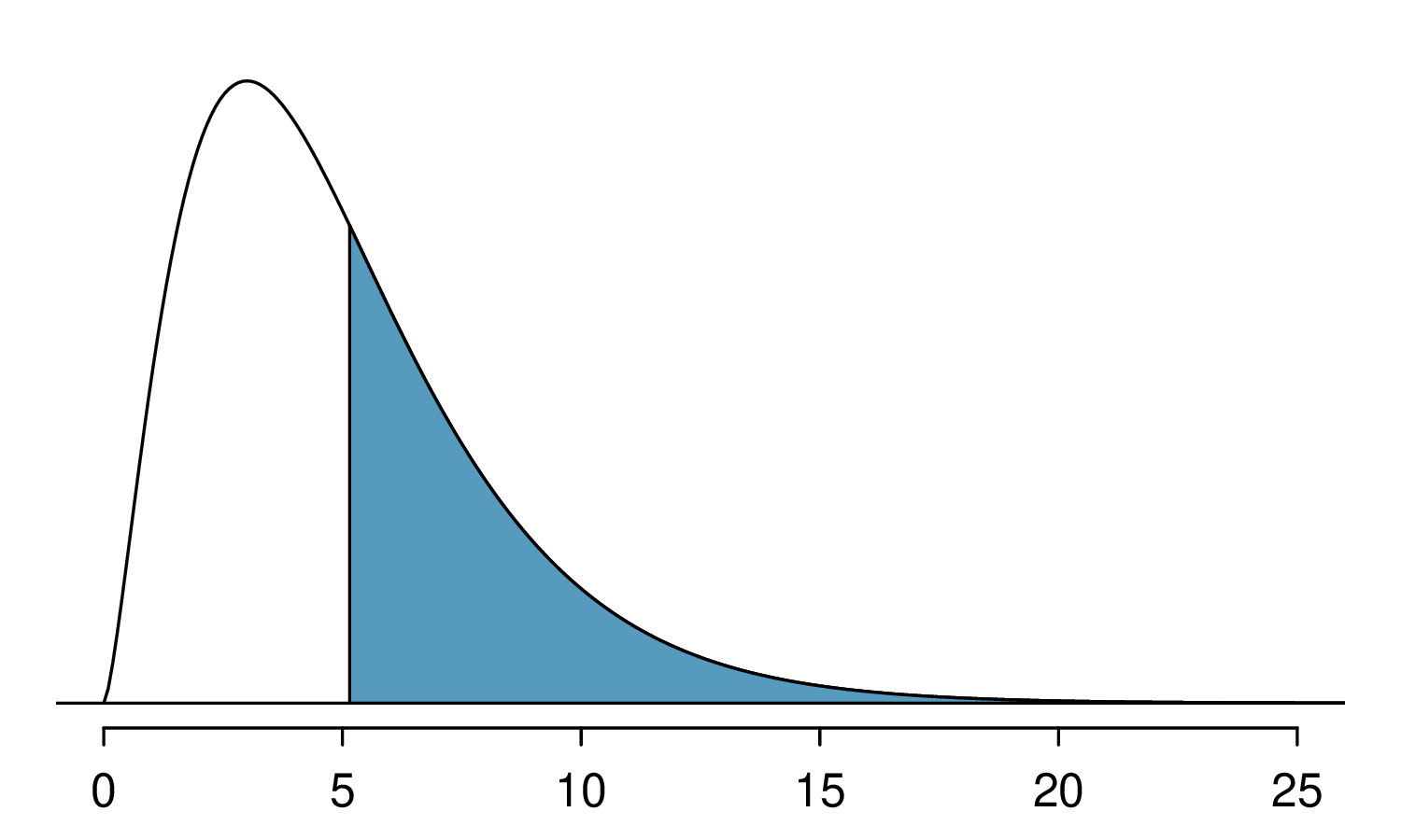
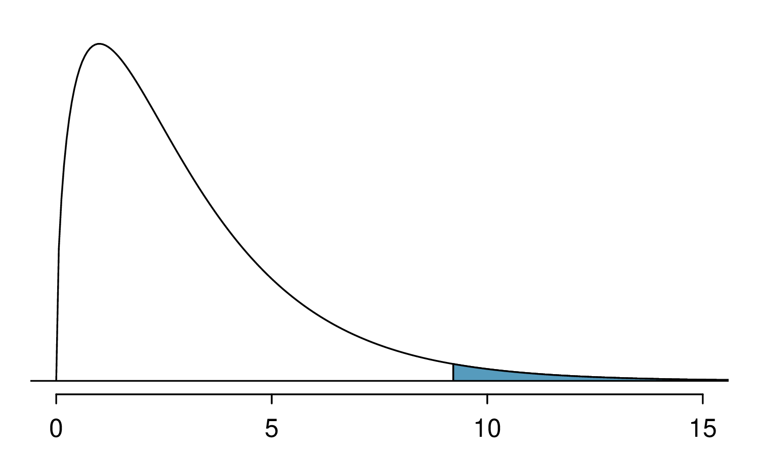
Using software, we would obtain a tail area of 0.4038. If using the table in Appendix C, we would have identified that the tail area is larger than 0.3 but not be able to give the precise value.

🔗

Checkpoint 6.3.11.

Figure 6.3.8(b) shows a cutoff of 11.7 on a chi-square distribution with 7 degrees of freedom. Find the area of the upper tail.

🔗

Solution.

The area is 0.1109. If using a table, we would identify that it falls between 0.1 and 0.2.

🔗

Checkpoint 6.3.12.

Figure 6.3.8(a) shows a cutoff of 10 on a chi-square distribution with 4 degrees of freedom. Find the area of the upper tail.

🔗

Solution.

Precise value: 0.0404. If using the table: between 0.02 and 0.05.

🔗

Checkpoint 6.3.13.

Figure 6.3.8(b) shows a cutoff of 9.21 with a chi-square distribution with 3 df. Find the area of the upper tail.

🔗

Solution.

Precise value: 0.0266. If using the table: between 0.02 and 0.05.

🔗

Subsection 6.3.4 Finding a p-value for a chi-square distribution

In Subsection 6.3.2, we identified a new test statistic (\(X^2\)) within the context of assessing whether there was evidence of racial bias in how jurors were sampled. The null hypothesis represented the claim that jurors were randomly sampled and there was no racial bias. The alternative hypothesis was that there was racial bias in how the jurors were sampled.

🔗

We determined that a large \(X^2\) value would suggest strong evidence favoring the alternative hypothesis: that there was racial bias. However, we could not quantify what the chance was of observing such a large test statistic (\(X^2=5.89\)) if the null hypothesis actually was true. This is where the chi-square distribution becomes useful. If the null hypothesis was true and there was no racial bias, then \(X^2\) would follow a chi-square distribution, with three degrees of freedom in this case. Under certain conditions, the statistic \(X^2\) follows a chi-square distribution with \(k - 1\) degrees of freedom, where \(k\) is the number of bins.

🔗

Example 6.3.14.

How many categories were there in the juror example? How many degrees of freedom should be associated with the chi-square distribution used for \(X^2\text{?}\)

🔗

Solution.

In the jurors example, there were \(k=4\) categories: White, Black, Hispanic, and other. According to the rule above, the test statistic \(X^2\) should then follow a chi-square distribution with \(k-1 = 3\) degrees of freedom if \(H_0\) is true.

🔗

Just like we checked sample size conditions to use a normal distribution in earlier sections, we must also check a sample size condition to safely apply the chi-square distribution for \(X^2\text{.}\) Each expected count must be at least 5. In the juror example, the expected counts were 198, 19.25, 33, and 24.75, all easily above 5, so we can apply the chi-square model to the test statistic, \(X^2=5.89\text{.}\)

🔗

Example 6.3.15.

If the null hypothesis is true, the test statistic \(X^2=5.89\) would be closely associated with a chi-square distribution with three degrees of freedom. Using this distribution and test statistic, identify the p-value.

🔗

Solution.

The chi-square distribution and p-value are shown in Figure 6.3.16. Because larger chi-square values correspond to stronger evidence against the null hypothesis, we shade the upper tail to represent the p-value. Using statistical software (or the table in Appendix C), we can determine that the area is 0.1171. Generally we do not reject the null hypothesis with such a large p-value. In other words, the data do not provide convincing evidence of racial bias in the juror selection.

🔗

A chi-square distribution with 3 degrees of freedom is shown, with the area above 5.89 shaded. This region appears to be about 10% of the area under the curve. — Figure 6.3.16. The p-value for the juror hypothesis test is shaded in the chi-square distribution with \(df=3\text{.}\)
🔗

Chi-square test for one-way table.

Suppose we are to evaluate whether there is convincing evidence that a set of observed counts \(O_1\text{,}\) \(O_2\text{,}\) ..., \(O_k\) in \(k\) categories are unusually different from what might be expected under a null hypothesis. Call the expected counts that are based on the null hypothesis \(E_1\text{,}\) \(E_2\text{,}\) ..., \(E_k\text{.}\) If each expected count is at least 5 and the null hypothesis is true, then the test statistic below follows a chi-square distribution with \(k-1\) degrees of freedom:

🔗

The p-value for this test statistic is found by looking at the upper tail of this chi-square distribution. We consider the upper tail because larger values of \(X^2\) would provide greater evidence against the null hypothesis.

🔗

Conditions for the chi-square test.

There are two conditions that must be checked before performing a chi-square test:

Independence. 🔗: Each case that contributes a count to the table must be independent of all the other cases in the table.
🔗
Sample size / distribution. 🔗: Each particular scenario (i.e. cell count) must have at least 5 expected cases.
🔗

🔗

Failing to check conditions may affect the test’s error rates.

🔗

When examining a table with just two bins, pick a single bin and use the one-proportion methods introduced in Section 6.1.

🔗

Subsection 6.3.5 Evaluating goodness of fit for a distribution

3.5 would be useful background reading for this example, but it is not a prerequisite.

🔗

We can apply the chi-square testing framework to the second problem in this section: evaluating whether a certain statistical model fits a data set. Daily stock returns from the S&P500 for 10 years can be used to assess whether stock activity each day is independent of the stock’s behavior on previous days. This sounds like a very complex question, and it is, but a chi-square test can be used to study the problem. We will label each day as Up or Down (D) depending on whether the market was up or down that day. For example, consider the following changes in price, their new labels of up and down, and then the number of days that must be observed before each Up day:

🔗

Table 6.3.17. Example sequence of daily price changes and waiting times.

🔗

Change in price	2.52	-1.46	0.51	-4.07	3.36	1.10	-5.46	-1.03	-2.99	1.71
Outcome	Up	D	Up	D	Up	Up	D	D	D	Up
Days to Up	1	-	2	-	2	1	-	-	-	4

If the days really are independent, then the number of days until a positive trading day should follow a geometric distribution. The geometric distribution describes the probability of waiting for the \(k^{th}\) trial to observe the first success. Here each up day (Up) represents a success, and down (D) days represent failures. In the data above, it took only one day until the market was up, so the first wait time was 1 day. It took two more days before we observed our next Up trading day, and two more for the third Up day. We would like to determine if these counts (1, 2, 2, 1, 4, and so on) follow the geometric distribution. Table 6.3.18 shows the number of waiting days for a positive trading day during 10 years for the S&P500.

🔗

Table 6.3.18. Observed distribution of the waiting time until a positive trading day for the S&P500.

🔗

Days		1	2	3	4	5	6	7+		Total
Observed		717	369	155	69	28	14	10		1362

We consider how many days one must wait until observing an Up day on the S&P500 stock index. If the stock activity was independent from one day to the next and the probability of a positive trading day was constant, then we would expect this waiting time to follow a geometric distribution. We can organize this into a hypothesis framework:

🔗

\(H_0\text{:}\) The stock market being up or down on a given day is independent from all other days. We will consider the number of days that pass until an Up day is observed. Under this hypothesis, the number of days until an Up day should follow a geometric distribution.

🔗
\(H_A\text{:}\) The stock market being up or down on a given day is not independent from all other days. Since we know the number of days until an Up day would follow a geometric distribution under the null, we look for deviations from the geometric distribution, which would support the alternative hypothesis.

🔗

There are important implications in our result for stock traders: if information from past trading days is useful in telling what will happen today, that information may provide an advantage over other traders.

🔗

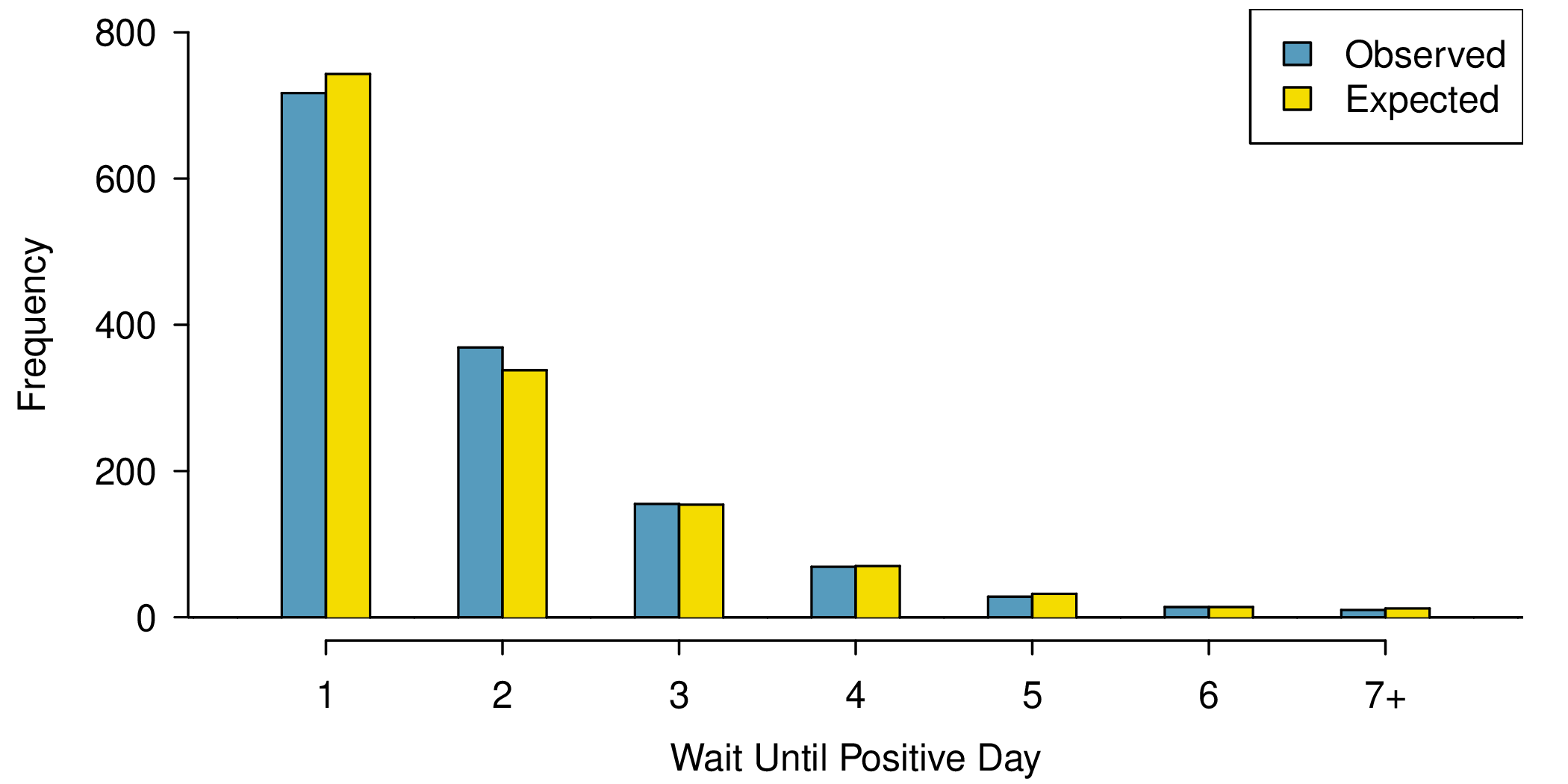
We consider data for the S&P500 and summarize the waiting times in Table 6.3.19 and Figure 6.3.20. The S&P500 was positive on 54.5% of those days.

🔗

Table 6.3.19. Distribution of the waiting time until a positive trading day. The expected counts based on the geometric model are shown in the last row. To find each expected count, we identify the probability of waiting \(D\) days based on the geometric model (\(P(D) = (1-0.545)^{D-1}(0.545)\)) and multiply by the total number of streaks, 1362. For example, waiting for three days occurs under the geometric model about \(0.455^2\times 0.545 = 0.1128 = 11.28\%\) of the time, which corresponds to \(0.1128 \times 1362 = 154\) streaks.

🔗

Days	1	2	3	4	5	6	7+	Total
Observed	717	369	155	69	28	14	10	1362
Geometric Model	743	338	154	70	32	14	12	1362

A side-by-side bar plot is shown for the variable "Wait Until Positive Day", where the two groups shown for the bars are "Observed counts" and "Expected counts". The horizontal axis shows values 1, 2, 3, 4, 5, 6, and "7+". The bar heights highest for "1" at roughly 715 for Observed and 740 for Expected. The bar heights for "2" are about half as high as at "1", with values of about 370 for Observed and 340 for Expected. The bar heights for "3" are about another half has high at about 150 for each for observed and expected. The values at 5, 6, and 7+ are all relatively small, at or below about 30. — Figure 6.3.20. Side-by-side bar plot of the observed and expected counts for each waiting time.
🔗

Because applying the chi-square framework requires expected counts to be at least 5, we have binned together all the cases where the waiting time was at least 7 days to ensure each expected count is well above this minimum. The actual data, shown in the Observed row in Table 6.3.19, can be compared to the expected counts from the Geometric Model row. The method for computing expected counts is discussed in Table 6.3.19. In general, the expected counts are determined by (1) identifying the null proportion associated with each bin, then (2) multiplying each null proportion by the total count to obtain the expected counts. That is, this strategy identifies what proportion of the total count we would expect to be in each bin.

🔗

Example 6.3.21.

Do you notice any unusually large deviations in the graph? Can you tell if these deviations are due to chance just by looking?

🔗

Solution.

It is not obvious whether differences in the observed counts and the expected counts from the geometric distribution are significantly different. That is, it is not clear whether these deviations might be due to chance or whether they are so strong that the data provide convincing evidence against the null hypothesis. However, we can perform a chi-square test using the counts in Table 6.3.19.

🔗

Checkpoint 6.3.22.

Table 6.3.19 provides a set of count data for waiting times (\(O_1=717\text{,}\) \(O_2=369\text{,}\) ...) and expected counts under the geometric distribution (\(E_1=743\text{,}\) \(E_2=338\text{,}\) ...). Compute the chi-square test statistic, \(X^2\text{.}\)

🔗

Solution.

\(X^2 = \frac{(717-743)^2}{743} + \frac{(369-338)^2}{338} + \cdots + \frac{(10-12)^2}{12} = 4.61\)

🔗

Checkpoint 6.3.23.

Because the expected counts are all at least 5, we can safely apply the chi-square distribution to \(X^2\text{.}\) However, how many degrees of freedom should we use?

🔗

Solution.

There are \(k = 7\) groups, so we use \(df = k - 1 = 6\text{.}\)

🔗

Example 6.3.24.

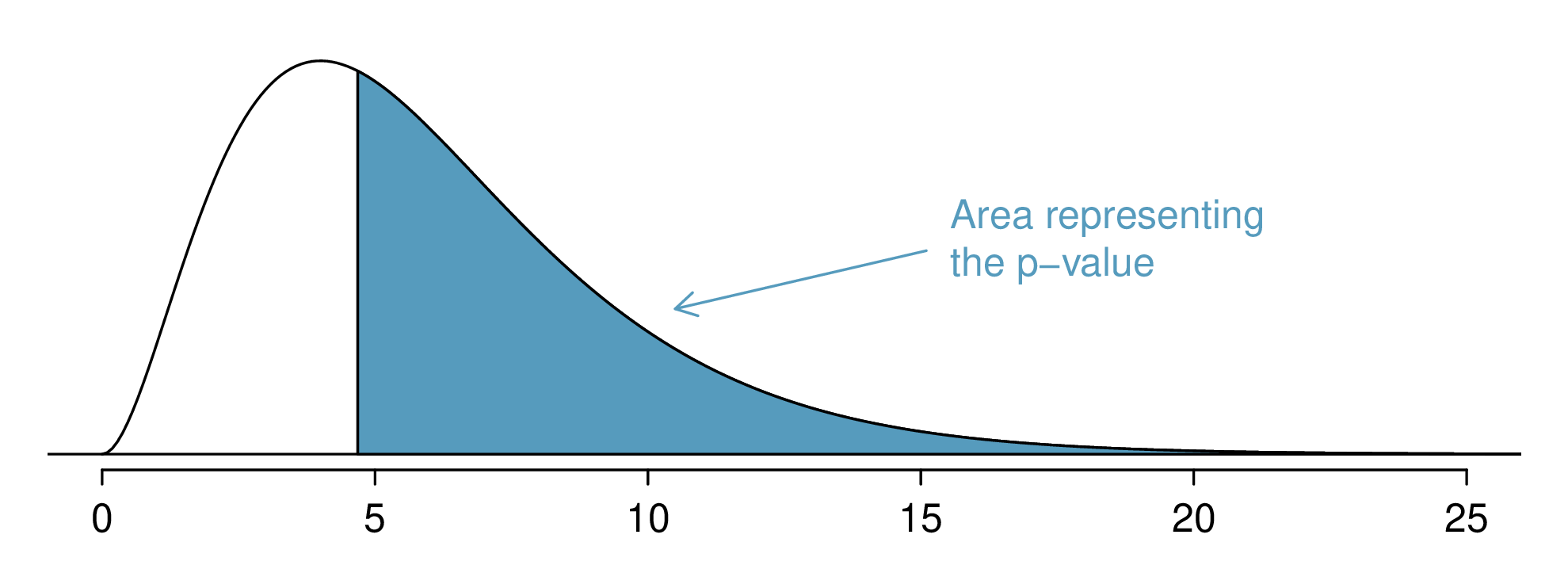
If the observed counts follow the geometric model, then the chi-square test statistic \(X^2 = 4.61\) would closely follow a chi-square distribution with \(df = 6\text{.}\) Using this information, compute a p-value.

🔗

Solution.

Figure 6.3.25 shows the chi-square distribution, cutoff, and the shaded p-value. Using software, we can find the p-value: 0.5951. Ultimately, we do not have sufficient evidence to reject the notion that the wait times follow a geometric distribution for the last 10 years of data for the S&P500, i.e. we cannot reject the notion that trading days are independent.

🔗

A chi-square distribution with 6 degrees of freedom is shown, with the area above 4.61 shaded. This region appears to be about 60% of the area under the curve. — Figure 6.3.25. Chi-square distribution with 6 degrees of freedom. The p-value for the stock analysis is shaded.
🔗

Example 6.3.26.

In Example 6.3.24, we did not reject the null hypothesis that the trading days are independent during the last 10 years of data. Why is this so important?

🔗

Solution.

It may be tempting to think the market is "due" for an Up day if there have been several consecutive days where it has been down. However, we haven’t found strong evidence that there’s any such property where the market is "due" for a correction. At the very least, the analysis suggests any dependence between days is very weak.

🔗

Exercises 6.3.6 Section 6.3 Exercises

1. True or false, Part I.

Determine if the statements below are true or false. For each false statement, suggest an alternative wording to make it a true statement.

🔗

The chi-square distribution, just like the normal distribution, has two parameters, mean and standard deviation.

🔗
The chi-square distribution is always right skewed, regardless of the value of the degrees of freedom parameter.

🔗
The chi-square statistic is always positive.

🔗
As the degrees of freedom increases, the shape of the chi-square distribution becomes more skewed.

🔗

🔗

2. True or false, Part II.

Determine if the statements below are true or false. For each false statement, suggest an alternative wording to make it a true statement.

🔗

As the degrees of freedom increases, the mean of the chi-square distribution increases.

🔗
If you found \(\chi^2 = 10\) with \(df = 5\) you would fail to reject \(H_0\) at the 5% significance level.

🔗
When finding the p-value of a chi-square test, we always shade the tail areas in both tails.

🔗
As the degrees of freedom increases, the variability of the chi-square distribution decreases.

🔗

🔗

3. Open source textbook.

A professor using an open source introductory statistics book predicts that 60% of the students will purchase a hard copy of the book, 25% will print it out from the web, and 15% will read it online. At the end of the semester he asks his students to complete a survey where they indicate what format of the book they used. Of the 126 students, 71 said they bought a hard copy of the book, 30 said they printed it out from the web, and 25 said they read it online.

🔗

State the hypotheses for testing if the professor’s predictions were inaccurate.

🔗
How many students did the professor expect to buy the book, print the book, and read the book exclusively online?

🔗
This is an appropriate setting for a chi-square test. List the conditions required for a test and verify they are satisfied.

🔗
Calculate the chi-squared statistic, the degrees of freedom associated with it, and the p-value.

🔗
Based on the p-value calculated in part (d), what is the conclusion of the hypothesis test? Interpret your conclusion in this context.

🔗

🔗

4. Barking deer.

Microhabitat factors associated with forage and bed sites of barking deer in Hainan Island, China were examined. In this region woods make up 4.8% of the land, cultivated grass plot makes up 14.7%, and deciduous forests make up 39.6%. Of the 426 sites where the deer forage, 4 were categorized as woods, 16 as cultivated grassplot, and 61 as deciduous forests. The table below summarizes these data.

🔗

Table 6.3.27. Barking deer forage sites by habitat type

🔗

Woods	Cultivated grassplot	Deciduous forests	Other	Total
4	16	61	345	426

Write the hypotheses for testing if barking deer prefer to forage in certain habitats over others.

🔗
What type of test can we use to answer this research question?

🔗
Check if the assumptions and conditions required for this test are satisfied.

🔗
Do these data provide convincing evidence that barking deer prefer to forage in certain habitats over others? Conduct an appropriate hypothesis test to answer this research question.

🔗

🔗

Prev Top Next